4 The Tidyverse
This chapter introduces the tidyverse. A series of packages, that helps us, to handle and manipulate data in R more easily.
4.1 Why not base R?
Many base R functions were written decades ago. They can be slow and the syntax may be clumsy. At the same time, it is difficult to change functions without breaking code, so most innovation occurs in new packages. The tidyverse is a collection of packages following a new and simple to use paradigm for handling data. Learn more at https://www.tidyverse.org.
The tidyverse is built around dplyr and its grammatical approach to data wrangling. It is also much faster than base R, as many dplyr functions export the actual computations to other fast languages in the background.
4.2 Some tidy conventions and concepts
Before we can use the tidyverse we have to install and load it. Run install.packages("tidyverse") to install the package (only once) and library() or require() to load the package (every timne you open R). Section 1.8 introduces packages in more detail.
install.packages("tidyverse")4.2.1 Tibbles
Tibbles are the preferred data format for using functions from the tidyverse. Any tibble is also a data frame, but not all data frames are tibbles. Let’s see this in practice:
i_df <- iris # built-in data
class(i_df)
#> [1] "data.frame"
i_tbl <- as_tibble(iris)
class(i_tbl)
#> [1] "tbl_df"     "tbl"        "data.frame"
One advantage is that tibbles only print the first 10 rows, and only as many columns as fit on your screen.
i_tbl # or print(i_tbl)
#> # A tibble: 150 × 5
#>    Sepal.Length Sepal.Width Petal.Length Petal.Width Species
#>           <dbl>       <dbl>        <dbl>       <dbl> <fct>
#>  1          5.1         3.5          1.4         0.2 setosa
#>  2          4.9         3            1.4         0.2 setosa
#>  3          4.7         3.2          1.3         0.2 setosa
#>  4          4.6         3.1          1.5         0.2 setosa
#>  5          5           3.6          1.4         0.2 setosa
#>  6          5.4         3.9          1.7         0.4 setosa
#>  7          4.6         3.4          1.4         0.3 setosa
#>  8          5           3.4          1.5         0.2 setosa
#>  9          4.4         2.9          1.4         0.2 setosa
#> 10          4.9         3.1          1.5         0.1 setosa
#> # ℹ 140 more rows
You can use tibbles like data frames:
i_tbl <- i_tbl[1:5,] # Subset the first 5 rows
i_tbl$Sepal.Length # Extract by name
#> [1] 5.1 4.9 4.7 4.6 5.0
i_tbl[["Sepal.Length"]] # Extract by name
#> [1] 5.1 4.9 4.7 4.6 5.0
i_tbl[[1]] # Extract by position
#> [1] 5.1 4.9 4.7 4.6 5.0
However, note the double squared brackets when subsetting tibbles, i.e. [[ ]] instaead of [ ].
Contrary to base R, subsetting variables with [ ] always returns another tibble:
i_tbl["Sepal.Length"] # or i_tbl[1]
#> # A tibble: 5 × 1
#>   Sepal.Length
#>          <dbl>
#> 1          5.1
#> 2          4.9
#> 3          4.7
#> 4          4.6
#> 5          5
Therefore, we use [[ ]] to extract the a vector:
i_tbl[["Sepal.Length"]] # or i_tbl[[1]]
#> [1] 5.1 4.9 4.7 4.6 5.0
Note, that not all functions work with tibbles. Therefore, you can always use
as.data.frame() to turn a tibble back to a data frame. In fact, the main reason that some older functions do not work with tibbles
is the [ function.
i_tbl <- as_tibble(iris)
i_df <- as.data.frame(i_tbl)
class(i_df)
#> [1] "data.frame"
Another difference is, that R functions usually use periods (.), whereas tidy functions use an
underscore (_).
4.2.2 Reading and Writing Data with Tibbles
The function read_csv is much faster and more convenient than base R and it does not convert strings to factors.
cps08 <- read_csv("data/cps08.csv")
print(cps08, n=2)
#> # A tibble: 7,711 × 5
#>     ahe  year bachelor female   age
#>   <dbl> <dbl> <chr>    <chr>  <dbl>
#> 1  38.5  2008 yes      no        33
#> 2  12.5  2008 yes      no        31
#> # ℹ 7,709 more rows
Use write_csv(cps08, "newfile.csv") for saving data. You may download the file cps08.csv from Stud.IP.
4.2.3 Tidy Data
R is so flexible, you can hold many data sets in memory and even make a data frame or list of data sets. Tidy data imposes some structure, just like STATA or Excel:
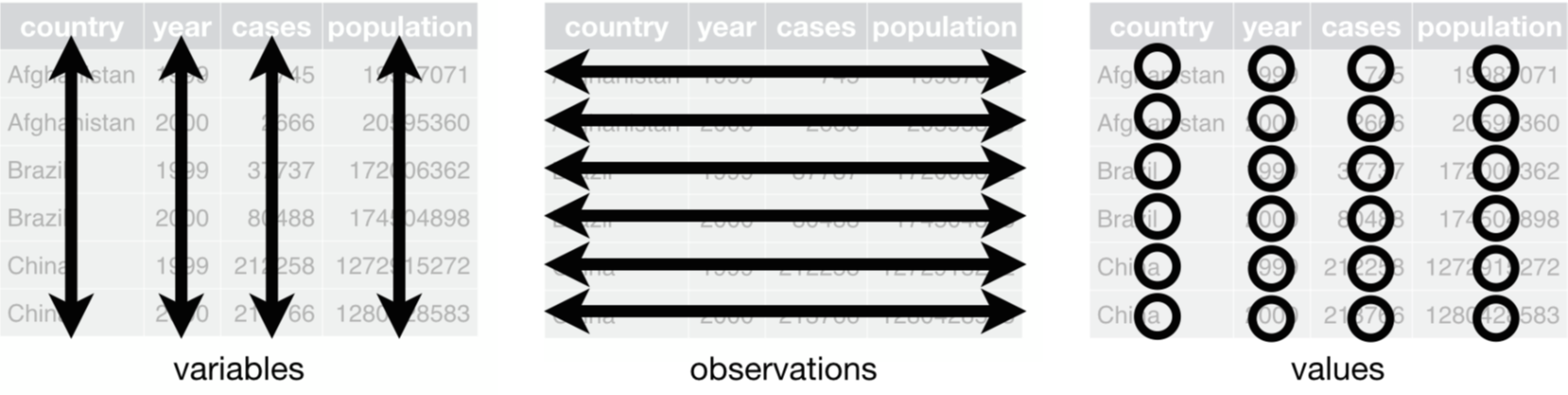
The following rules apply:
- Each variable must have its own column
- Each observation must have its own row
- Each value must have its own cell
4.3 Handling and Manipulating tidy Data
4.3.1 Subsetting Data with dplyr
Subsetting variables is easy using dplyr’s select() function:
select(cps08, bachelor)
#> # A tibble: 7,711 × 1
#>   bachelor
#>   <chr>
#> 1 yes
#> 2 yes
#> # ℹ 7,709 more rows
Note, that dplyr auto-“quotes” function inputs for you. select() has a large variety of convenience functions where you want to quote, e.g. starts_with(), ends_with(), or contains()
Subsetting columns is just as easy using the filter() function:
filter(cps08, age==33)
#> # A tibble: 720 × 5
#>     ahe  year bachelor female   age
#>   <dbl> <dbl> <chr>    <chr>  <dbl>
#> 1  38.5  2008 yes      no        33
#> 2  29.8  2008 yes      no        33
#> # ℹ 718 more rows
You can use all standard operators ==, >, >=, &, |, ! or functions is.na(), but also functions like between(x, left, right).
The arrange() function is used to reorder (or sort) rows according to one or more variable(s). Use desc(varname) to sort a variable in descending order:
arrange(cps08, year, bachelor, female, age)
#> # A tibble: 7,711 × 5
#>     ahe  year bachelor female   age
#>   <dbl> <dbl> <chr>    <chr>  <dbl>
#> 1 11.8   2008 no       no        25
#> 2  8.65  2008 no       no        25
#> # ℹ 7,709 more rows
4.3.2 Renaming Variables with dplyr
Renaming variables is horribly complicated in base R, but super
simple using rename():
rename(cps08, lohn=ahe, jahr=year, uni=bachelor,
       frau=female, alter=age)
#> # A tibble: 7,711 × 5
#>    lohn  jahr uni   frau  alter
#>   <dbl> <dbl> <chr> <chr> <dbl>
#> 1  38.5  2008 yes   no       33
#> 2  12.5  2008 yes   no       31
#> # ℹ 7,709 more rows
You can also just use new_name = old_name when calling select().
4.3.3 Changing Variables with dplyr
Changing variables is annoying in base R, but easy using the mutate() function. Note, that mutate() returns the entire data, transmute() only the transformed variable(s).
4.4 Grouping and Summarizing Data
A lot of analysis and data wrangling in social science applications is done in groups. A key feature of the dplyr package is its grouping and summarizing capabilities. dplyr provides us with easy-to-use functions group_by() and summarise or summarize. After grouping, summarize() will collapse the data accordingly:
cps08_grpd <- group_by(cps08, female, bachelor)
summarize(cps08_grpd, mean(ahe))
#> # A tibble: 4 × 3
#> # Groups:   female [2]
#>   female bachelor `mean(ahe)`
#>   <chr>  <chr>          <dbl>
#> 1 no     no              16.6
#> 2 no     yes             25.0
#> # ℹ 2 more rowsNote: The index in group_by() is sticky until you call ungroup().
Both, summarize() and mutate() play well with other dplyr functions:
-
first(),last()andnth() -
n()andn_distinct()
But also with base R functions:
You can also get summary statistics for all columns using summarise_all(cps08, funs(mean)).
4.4.1 The %>% pipe operator
Pipes are a powerful tool for clearly expressing a sequence of multiple operations. Press Ctrl + Shift + M to insert a pipe. Let’s group again:
cps08 %>% group_by(female, bachelor) %>%
  summarize(mean(ahe))
#> # A tibble: 4 × 3
#> # Groups:   female [2]
#>   female bachelor `mean(ahe)`
#>   <chr>  <chr>          <dbl>
#> 1 no     no              16.6
#> 2 no     yes             25.0
#> # ℹ 2 more rows
The Magrittr pipe %>% vs. the native pipe operator |>
After the success story of the pipe operator from the magrittr package, a native pipe was introduced, |>. They may seem to work the same for most functions, but they are not exactly the same. After working with both, we recommend to use the Magrittr pipe.
When not to use the pipe
The pipe is a powerful tool, but it does not solve every problem! Pipes are most useful for rewriting a fairly short linear sequence of operations.
Do not use when:
- Your pipes are getting very long. Create intermediate objects instead.
- You have multiple inputs or outputs. If there is no primary object, do not use pipes.
- You have some complex dependency structure. Pipes are fundamentally linear.
4.4.2 New Variables by Groups
Using group_by() with mutate() also summarizes data and simultaneously creates new variables. In this case, the data will not be collapsed:
4.4.3 Manipulating several variables at the same time
Often we would like to change several variables in the same way. The function across() offers an elegant solution to do this.
Assume we would like to change both, the bachelor and the female variable form the cps08.csv into numeric dummies. We name the variables that we would like to change as a vector (remember the auto quote). As an arguement we place the function that we would like to perform on the mentioned variables, using the tilde function ~.
cps08 <- cps08 %>%
  mutate(across(c(bachelor, female), ~if_else(.x == "yes",1,0)))
head(cps08)
#> # A tibble: 6 × 6
#>     ahe  year bachelor female   age ahe_group
#>   <dbl> <dbl>    <dbl>  <dbl> <dbl>     <dbl>
#> 1  38.5  2008        1      0    33      25.0
#> 2  12.5  2008        1      0    31      25.0
#> # ℹ 4 more rows
Note, that you have to use the .x as a place holder for the varialbes you would like to manipulate.
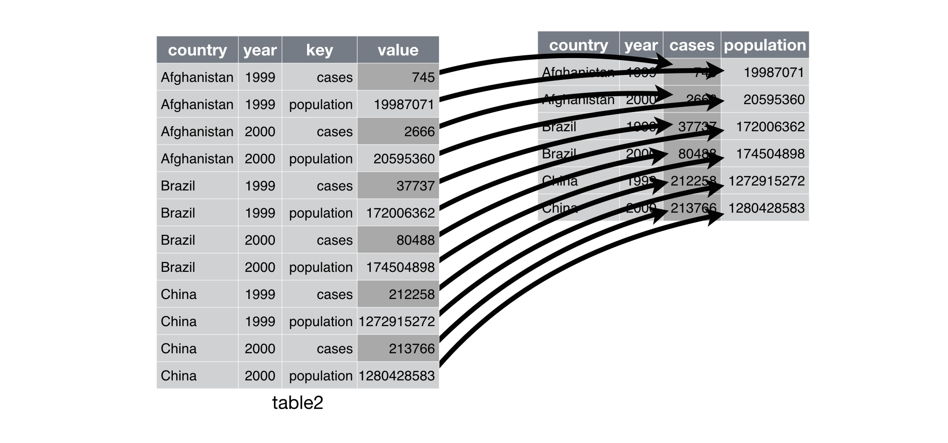
4.4.4 Reshaping Data
Most tidy functions require data in long (or tidy) format instead of a wide format. However, data is often organised to facilitate some use other than analysis, e.g. data is organised to make entry as easy as possible. Two major problems stem from this:
- One variable might be spread across multiple columns
- One observation might be scattered across multiple rows
Typically, a dataset will only suffers from one of these problems. To fix this, you need: pivot_longer() and pivot_wider(), that will reshape our data to long or wide format, respectively.
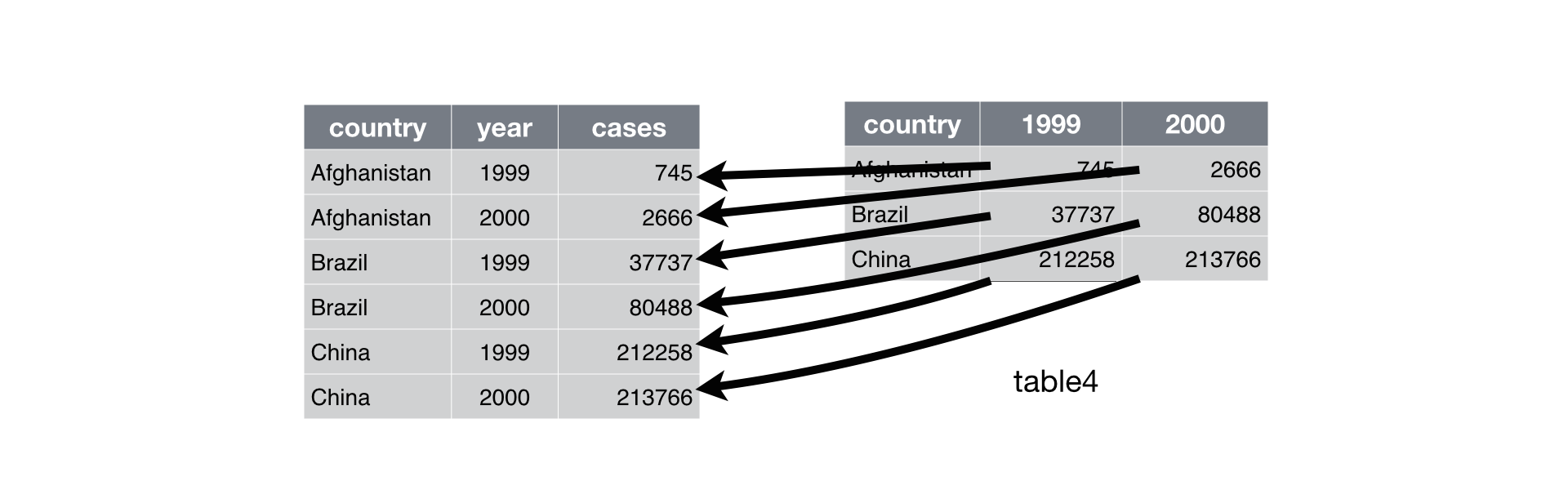
Let’s try to transpose our data in practice:
table4a # laod some data
#> # A tibble: 3 × 3
#>   country     `1999` `2000`
#>   <chr>        <dbl>  <dbl>
#> 1 Afghanistan    745   2666
#> 2 Brazil       37737  80488
#> # ℹ 1 more row

table4a %>% # turn wide data to long data
  pivot_longer(c(`1999`, `2000`),
               names_to = "year", values_to = "cases")
#> # A tibble: 6 × 3
#>   country     year  cases
#>   <chr>       <chr> <dbl>
#> 1 Afghanistan 1999    745
#> 2 Afghanistan 2000   2666
#> # ℹ 4 more rows
4.5 Saving tidy Data
Saving and loading data in R’s native binary format R has its own native binary format: RDS. You can store the entire work space (not recommended) or single objects (recommended)
You can save and load an object using the write_rds() and read_rds() functions, respectively:
# from tidyverse, or use base *R* saveRDS()
write_rds(cps08, file = "cps08.rds")

# from tidyverse, or use base *R* readRDS()
cps08 <- read_rds("cps08.rds")
Use RDS if you will continue using the file in R and do not want to lose auxiliary information about the data (e.g. group_by keys).
4.6 Using Data in Other Binary Formats
The haven-package is part of the tidyverse and reads/writes STATA, SPSS or SAS files:
require(haven)
path <- system.file("examples", "iris.dta",
                    package = "haven")
my_tbl <- read_dta(path)
readxl is also part of the tidyverse and reads/writes Excel files:
require(readxl)
xlsx_example <- readxl_example("datasets.xlsx")
my_tbl <- read_excel(xlsx_example, sheet = "mtcars")
4.7 Exercise: Tidyverse
Load the movie ratings data set from http://www.stern.nyu.edu/~wgreene/Text/Edition7/TableF4-3.csv. Try to run all operations in tidyverse style.
- Select the first five variables only. Change the variable BOX which measures the box office return in USD to millions.
- Create a new factor called MPAA from MPRATING with the levels 1=G, 2=PG, 3=PG13, and 4=R.
- Compute the average
BOX,BUDGET, andBOX/BUDGETratio for eachMPAAvalue. Which rating class recovers most of the initial investment during the first US run? - Join this data back to the original data frame. Find the top 6 over and under-performers as measured in deviations from the box office over budget ratio in each class.
- Could you have done 3. and 4. directly in the tibble without using a join? If so, do it and show that it is equivalent.
Answer
# Solution Exercise tidyverse

#Load the movie ratings data set from www.stern.nyu.edu/~wgreene/Text/Edition7/TableF4-3.csv.
# Do all operations in tidyverse style.

rm(list = ls())
require(tidyverse)
url <- "http://www.stern.nyu.edu/~wgreene/Text/Edition7/TableF4-3.csv"
movies_tbl <- read_csv(url)

# 1. Select the first five variables only. Change the variable BOX which measures the box office
# return in US$ to millions.

movies_tbl <- movies_tbl %>% select(1:5)
movies_tbl <- movies_tbl %>% mutate(BOX = BOX/1e6)

# 2. Create a new factor called MPAA from MPRATING with the levels 1=G, 2=PG, 3=PG13, and 4=R.
movies_tbl <- movies_tbl %>% mutate(MPAA = factor(MPRATING, levels = c(1,2,3,4),
                                                  labels = c("G", "PG", "PG13", "R")))

# 3. Compute the average BOX, BUDGET, and BOX/BUDGET ratio for each MPAA value.
# Which rating class recovers most of the initial investment during the first US run?

sum_tbl <- movies_tbl %>% group_by(MPAA) %>%
  summarize(MBUDGET = mean(BUDGET),
            MBOX = mean(BOX),
            MRATIO = mean(BOX/BUDGET))
sum_tbl

# 4. Join this data back to the original data frame. Find the top 6 over and under-performers
# as measured in deviations from the box office over budget ratio in each class.

full_tbl <- movies_tbl %>% left_join(sum_tbl, by="MPAA") %>%
  mutate(PERFOR = BOX/BUDGET - MRATIO)

# top and bottom 6
head(full_tbl %>% arrange(PERFOR))

# descending order
head(full_tbl %>% arrange(desc(PERFOR)))

# 5. Could you have done 3. and 4. directly in the tibble without using a join? If so, do it and
# show that it is equivalent.

movies_tbl <- movies_tbl %>% group_by(MPAA) %>%
  mutate(MBUDGET = mean(BUDGET),
         MBOX = mean(BOX),
         MRATIO = mean(BOX/BUDGET)) %>%
  mutate(PERFOR = BOX/BUDGET - MRATIO) %>% ungroup()
head(movies_tbl %>% arrange(PERFOR))

# or use
movies_tbl %>% arrange(desc(PERFOR)) %>% head()
4.8 Appendix: Other useful dplyr-verbs:
Reshaping data:
-
separate()one column into several -
unite()several columns into one -
distinct()removes duplicates
Combining data:
-
bind_rows(y, z)appendztoyas new rows -
bind_cols(y, z)appendztoyas new columns -
left_join(a, b, by = "ID_1")matching rows frombtoa -
right_join(a, b, by = "ID_1")matching rows fromatob -
inner_join(a, b, by = "ID_1")retain only rows in both sets -
full_join(a, b, by = "ID_1")retain all matching rows/ values -
across()manipulate several variables at the same time