2 R Basics

In this chapter, we learn the basic concepts and paradigms on which R builds. We get to know all essential object and data types. Further, we learn how to manipulate data in R, using standard functions and syntax.

2.1 Basic R Objects

2.1.1 Atomic Objects

R knows five types of atomic objects:

numeric objects are all real numbers on a continuous scale [e.g. 1.23456].
integer are all full numbers [e.g. 1, typed as 1L]. If you want an integer you have to explicitly, use the L suffix. Otherwise, R will assign the number to the numeric class.
complex is used for complex numbers [e.g.a + bi, i.e. real + imaginary].
boolean values are logical values like TRUE and False.
strings are characters [e.g. "Hello World!"]. Use the ' or the ". Note that all other atomic objects can be converted into strings.

The data types collecting these atomic objects are:

Vectors: several elements of a single atomic type
- (R does not have scalars, they are 1-element vectors)
Matrices: collections of equal-length vectors
Factors: categorical data (ordered, unordered)
Data frames: a data set, collections of equal-length vectors of different types
Lists: collections of unequal-length vectors of different types

2.1.2 Vectors of Atomic Objects

R automatically assigns the correct object type. Let’s look at this in practice:

x <- c(1.1, 2.2, 3.3)
is.numeric(x)
#> [1] TRUE
x <- c(1L, 2L, 3L)
is.integer(x)
#> [1] TRUE
x <- c(1+0i, 2+4i, 3+6i)
is.complex(x)
#> [1] TRUE
x <- c(TRUE, FALSE, TRUE)
is.logical(x)
#> [1] TRUE
x <- c("I", "like", "R")
is.character(x)
#> [1] TRUE

2.2 Missing and Other Special Values

Missing values can be of any atomic type. R has designated signs for “not available” (NA), not a number (NaN), positive infinity (Inf), and negative infinity (-Inf).

Missing values are denoted by NA or NaN for undefined mathematical operations. NA values have a class also, so there are integer NA, character NA, etc. The value NaN represents an undefined value, e.g. 0/0. Note, this implies that an NaN value is also NA, but the inverse is not true!

In addition to missing values, R also defines a special number Inf which represents infinity (and -Inf for minus infinity, respectively). This allows us to represent entities like 1/0 and Inf can be used in ordinary calculations, e.g. 1 / Inf = 0.

Let’s look at these special cases in practice:

1/0 # infinity
#> [1] Inf
log(0) # negative infinity
#> [1] -Inf
c("yes", NA) # not available
#> [1] "yes" NA
0/0 # not a number
#> [1] NaN

Various is.X() functions are available to look for special value entries in vectors:

a <- c(NA, NaN, Inf)
is.na(a)
#> [1]  TRUE  TRUE FALSE
is.nan(a)
#> [1] FALSE  TRUE FALSE
is.infinite(a)
#> [1] FALSE FALSE  TRUE

Activity

What data type is this vector? x <- c("R", 2, FALSE)
What data type is this vector? x <- c(2, FALSE)

2.3 Matrices

Matrices are collections of vectors. The dimensions are \(r \times k\), where \(r\) is the number of rows and \(k\) is the number of columns. Note, that the input vectors have to be of equal length and equal type.

Let’s create our own matrix:

x1 <- 1:3
x2 <- 4:6
x3 <- 7:9
x <- cbind(x1,x2,x3)
x
#>      x1 x2 x3
#> [1,]  1  4  7
#> [2,]  2  5  8
#> [3,]  3  6  9

We can inspect our matrix, x, using the dim() function which returns the dimensions of the matrix. The length() functions reports the length of the matrix, i.e. \(r \times k\).

dim(x) ## returns r and k
#> [1] 3 3
length(x) ## returns r times k
#> [1] 9

To create a matrix, we can also break a long vector into rows and columns:

m <- matrix(1:9, ncol = 3, nrow = 3)
m
#>      [,1] [,2] [,3]
#> [1,]    1    4    7
#> [2,]    2    5    8
#> [3,]    3    6    9

You can perform mathematical operations on matrices at will, however, note that simple mathematical operations are performed element wise for matrices:

m*m
#>      [,1] [,2] [,3]
#> [1,]    1   16   49
#> [2,]    4   25   64
#> [3,]    9   36   81

For matrix algebra, use special functions, such as %*% for matrix multiplication or t() for the transpose.

2.4 Factors

Factors store categorical data that may be ordered or unordered. This can be, for example, binary "yes" and "no", ordinal like "disagree", "neutral" and "agree", or just unordered car brands like "BMW", "Mercedes", and "Volkswagen".

Let’s inspect factors in practice:

x <- factor(c("yes", "yes", "no", "yes", "no"))
x # The factor assigned two levels, one for `"yes"` and one for `"no"`. 
#> [1] yes yes no  yes no 
#> Levels: no yes
table(x)
#> x
#>  no yes 
#>   2   3

Factors are very useful, but they also have their pitfalls. Therefore, only use factors when you need them! Often, R assigns string data as factors automatically, so make sure to check that you work with string data if you want to.

Factors usually have an intrinsic order (for example a Likert scale). You can alter the order of the levels using the levels argument.

x <- factor(c("agree", "agree", "neutral"),
      levels = c("disagree", "neutral", "agree"))
x
#> [1] agree   agree   neutral
#> Levels: disagree neutral agree
unclass(x) # shows how it's really stored
#> [1] 3 3 2
#> attr(,"levels")
#> [1] "disagree" "neutral"  "agree"

2.5 Data Frames

Data frames are the most important data type for statistical analysis in R. They can hold all atomic types, provided they are in vectors of equal length. You can think of data frames as an excel sheet or a table that records different characteristics for different units of observations. In fact, STATA can only open one data frame at a time. In R you can open and check as many data frames as your machine has memory.

Let’s create our own data frame:

x <- data.frame(id = 1:5, male = c(T, T, F, F, F),
                  age = c(29, 45, 23, 62, 59))
x
#>   id  male age
#> 1  1  TRUE  29
#> 2  2  TRUE  45
#> 3  3 FALSE  23
#> 4  4 FALSE  62
#> 5  5 FALSE  59

2.6 Lists

Lists are the most flexible data form in R. They can hold any type of vector consisting of different atomic elements and of different length. They are a very powerful tool, especially for programming, but their extreme flexibility makes it more challenging to handle them. Due to its structure, you can easily loose track of what exactly is stored in a list you just created.

Let’s see lists in practice:

mylist <- list(beers = c("Pils", "Lager",
                         "Pale Ale", "Dark Ale"),
               cars = c("BMW", "Mercedes", "VW"),
               numbers = c(1:5))
mylist
#> $beers
#> [1] "Pils"     "Lager"    "Pale Ale" "Dark Ale"
#> 
#> $cars
#> [1] "BMW"      "Mercedes" "VW"      
#> 
#> $numbers
#> [1] 1 2 3 4 5

Exercise 2

Question 1: Vectors and Matrices

Copy the following code lines and create the 3 different outputs below. Hint: Use the functions rbind(), cbind() and c()

x1 <- 1:3
x2 <- 4:6
x3 <- 7:9

Outputs:

#>      x1 x2 x3
#> [1,]  1  4  7
#> [2,]  2  5  8
#> [3,]  3  6  9
#>    [,1] [,2] [,3]
#> x1    1    2    3
#> x2    4    5    6
#> x3    7    8    9
#> [1] 1 2 3 4 5 6 7 8 9

Answer

# Question 1: Change the default argument in a function
x1 <- 1:3
x2 <- 4:6
x3 <- 7:9
x <- cbind(x1,x2,x3)
x
x <- rbind(x1,x2,x3)
x
x <- c(x1,x2,x3)
x

Question 2: NA, NaN, Null

Run the following lines of code:

a <- c(rep(1, runif(1, min=0,max=100))
       , rep(NA, runif(1, min=0,max=100)))
b <- c(rep(1, runif(1, min=0,max=100))
       , rep(NaN, runif(1, min=0,max=100)))
c <- c(rep(1, runif(1, min=0,max=100))
       , rep(NULL, runif(1, min=0,max=100)))

Dissect the line creating the first object to understand what each sub-command is doing.
Let R display the length of each vector only containing numbers.
- Hint: Use the length() command to display the number of observations in a vector.
- Use an is.X command to display the number of special values.

Answer

## Question 1: NA, NaN, NULL
a <- c(rep(1, runif(1, min=0,max=100))
       , rep(NA, runif(1, min=0,max=100)))
b <- c(rep(1, runif(1, min=0,max=100))
       , rep(NaN, runif(1, min=0,max=100)))
c <- c(rep(1, runif(1, min=0,max=100))
       , rep(NULL, runif(1, min=0,max=100)))

?rep
?runif

## Getting the length of vector a
### alternative 1
nas <- a[is.na(a)]
length(a) - length(nas)

# alternative 2
length(a) - length(a[is.na(a)]) 

# alternative 3
length(a) - sum((is.na(a)))

# alternative 4
length(a[!is.na(a)])

2.7 Operations with Objects in R

We just learned about a couple of object types: Vectors, matrices, data frames, lists, etc. R is all about applying functions to these objects. While most functions work with most object types, there are certain differences. If you are unsure which object a function needs, you can check the help file.

2.7.1 Operations with Vectors

To subset a vector use the [] brackets:

x <- 1:10
x[1:5]
#> [1] 1 2 3 4 5

Most functions work on a vector, e.g. statistical functions:

mean(x) # mean
#> [1] 5.5
sd(x) # standard deviation
#> [1] 3.02765
var(x) # variance
#> [1] 9.166667
length(x) # length
#> [1] 10
sum(x) # sum
#> [1] 55

The same also works for subsets of vectors:

x[1:5]
#> [1] 1 2 3 4 5
mean(x[1:5]) # mean over a subset
#> [1] 3

R by default does vector operations element-wise. This requires equally sized vectors (or multiples). Note, that for vector algebra we have to use a different notation (advanced use).

a <- 1:10
b <- 11:20
a + b
#>  [1] 12 14 16 18 20 22 24 26 28 30

Recycling: If vectors are not equally sized, but one is a multiple of the other, R “recycles” the shorter one:

a <- c(1,1,1,1)
b <- c(2,4)
a * b
#> [1] 2 4 2 4

Note: R recycles vectors only!

2.7.2 More on Recycling

R applies its recycling also when we apply functions to vectors together with other data types:

a <- matrix(1:8,nrow=2,ncol=4)
b <- c(10,20)

a*b
#>      [,1] [,2] [,3] [,4]
#> [1,]   10   30   50   70
#> [2,]   40   80  120  160
rbind(a,b)
#>   [,1] [,2] [,3] [,4]
#>      1    3    5    7
#>      2    4    6    8
#> b   10   20   10   20

However, when we try to combine two matrices, R returns an error:

a <- matrix(c(1,2,3,4),2,2)
b <- matrix(c(1:8),2,4)

#This would produce an error:
#a+b
cbind(a,a)+b
#>      [,1] [,2] [,3] [,4]
#> [1,]    2    6    6   10
#> [2,]    4    8    8   12

Exercise 3

Run the following code

a <- c(NA, "You", NaN, "XYZ" ,"happy", "Whatever"
       , 2, "That","I", "b", "so", "This", "Time"
       , "a", "am", "pm", "an")

Run separate commands each time to show one element of the vector only. Isolate elements 9,15,11,5.

Answer

# Question 2: Subsetting vectors
a <- c(NA, "You", NaN, "XYZ" ,"happy", "Whatever"
       , 2, "That","I", "b", "so", "This", "Time"
       , "a", "am", "pm", "an")
a[9]
a[15]
a[11]
a[5]

2.7.3 Naming Objects

All R data objects can be assigned names with the names(), the colnames(), or the rownames() functions. For data frames column names are very important, as they correspond to the variable name.

x <- data.frame(id = 1:5, male = c(T, T, F, F, F),
                age = c(29, 45, 23, 62, 59))
names(x) ##print names
#> [1] "id"   "male" "age"
## let's rename
names(x) <- c("personID", names(x)[-1])
names(x)[names(x) == "male"] <- "notfemale"
names(x)
#> [1] "personID"  "notfemale" "age"

2.8 Looking at Data Types

For all data types, it helps getting an overview of their content. Let us create a vector, by randomly taking 20 draws from strings and numeric entries, using the sample() function. unique() returns unique objects in our object a, while sort() arranges the data. set.seed() makes sure that our draw can be replicated.

set.seed(123)
a <- sample(c("YES","NO","MAYBE","HANNOVER","GOETTINGEN",
          "HAMBURG", 1:50),20,replace=T)
unique(a)[1:7] # Which entries do we have?
#> [1] "25"    "9"     "45"    "8"     "MAYBE" "36"    "44"
sort(table(a),decreasing = T)[1:6] # And how often?
#> a
#> 21 45 48  8 19 20 
#>  2  2  2  2  1  1
"HANNOVER" %in% a # Is a specific one included?
#> [1] FALSE

2.9 Combining Data Types

We can combine several data types to a data frame. To add rows we use the cbind() function, to add rows we use rbind().

# create a data frame:
fb <- data.frame(city=c("Stuttgart","Muenchen","Dortmund"),
                club=c("VfB","FCB","BVB"),
                stringsAsFactors = F)
#Add another column:
fb <- cbind(fb,rank=c(13,18,4),league=1)
#Add more rows. Note that Colnames must match!
fb <- rbind(fb,data.frame(city=c("Berlin","Bielefeld"),
      club=c("Union","Arminia"),rank=c(8,1),league=1))
fb
#>        city    club rank league
#> 1 Stuttgart     VfB   13      1
#> 2  Muenchen     FCB   18      1
#> 3  Dortmund     BVB    4      1
#> 4    Berlin   Union    8      1
#> 5 Bielefeld Arminia    1      1

2.10 Working with Lists

Lists are special, because they allow you to store anything in them, even of totally different data types:

#T his opens an empty list of desired size
my.list <- as.list(rep(NA,times=4))

#Now we fill it element by element
my.list[[1]] <- c("This","Is","A","Vector")
my.list[[2]] <- data.frame(Data=1:5,Names=c("one","two",
                            "three","four","five"))
my.list[[3]] <- as.factor(c("YES","NO","YES","YES","NO",
                            "YES","NO","NO"))
my.list[[4]] <- list("We",c("can","even","put"),
                     data.frame(another=1:5,list=6:10))

To unpack a list directly however, we need data of the same type. The unlist() function flattens the list and returns a single vector. The do.call() function returns a matrix, but uses recycling to create objects of equal length.

a <- 1:2
b <- 3:4
c <- 5:8
my.list <- list(a,b,c)

unlist(my.list) # flattens a list into a singe vector
#> [1] 1 2 3 4 5 6 7 8
do.call(cbind, my.list) # Note the recycling!
#>      [,1] [,2] [,3]
#> [1,]    1    3    5
#> [2,]    2    4    6
#> [3,]    1    3    7
#> [4,]    2    4    8

Exercise 4

Question 1: Basic Functions

Run the following code to load some time series data on the body temperature of two beavers:

data(beavers)
my.data <- beaver1
# attach stores the vectors of the data frame directly in your workspace:
attach(my.data)

Now we have some data to work with.

Check the data frame’s column names. These are now the names of your vectors.
Over how many days did they follow the beaver’s temperature?
How many observations per day do we have?
Did they check temperature at 12pm?
Check the distribution of the temperature. What is the mean and the standard deviation?
During how many observations was the beaver active?

Answer


### 1. Basic Functions ###

# 1. Check the data frame's colnames. These are now the names of your vectors 
colnames(my.data)

# 2. Over how many days did they follow the beaver's temperature?
unique(day)
length(unique(day))

# 3. How many observations per day do we have?
unique(time)
table(day)

# 4. Did they check at 12pm?
1200 %in% time

# 5. Check the distribution of the temperature. Whats the mean and SD?
mean(temp)  
sd(temp)  

# 6. During how many observations was the beaver active?
table(activ)

Question 2: Combining Data

After the attach() function, we could use detach() to put all the variables back together to a data frame. To get some R-practice however, let’s build our beaver-data frame back together manually.

Use cbind() to combine the vectors and convert the matrix to a data frame. Don’t forget to assign the column names!
The dataset we loaded contains information about a second beaver too (beaver2). Create an ID variable for each beaver and add it to each data frame.
use rbind() to combine both data frames, in order to create a new data frame containing information about both beavers.

Answer

### Question 2: Combining Data ###

# Use `cbind()` to combine the vectors...
df <- cbind(day,time,temp,activ)

# ...and convert the matrix to a data frame. 
df <- data.frame(df)

# And don't forget to assign the Column-Names!  
colnames(df) <- c("day","time","temp","activ")

# Create two new objects containing an identifier...
bv1.id <- 1
bv2.id <- 2

# ...and add them to the dataframes. 
df <- cbind(df,bv1.id) # alternative: df <- cbind(beaver1,bv1.id)
df2 <- cbind(beaver2,bv2.id)

# then, combine both using `rbind()`
colnames(df) <- colnames(df2) <- c(colnames(df)[-5],"beaverID")
df <- rbind(df,df2)

Question 3: From Data to List to DataFrame…

Start by creating some random data:

a <- rnorm(50)
b <- rnorm(100)
c <- rnorm(200)
d <- sample(1:1000,50)
e <- sample(1:999999,400)

Now, open a list that contains all these vectors. Give the list names that allow you tracing back where your data entries come from.
We want to get from this list to a dataframe. First, make some theoretical considerations:

How should the dataframe look like in the end?
How many rows and columns should it have?
How could R’s recycling help or trick you here?

Let’s write some code. You saw two options to get rid of a list in the slides - which one does the trick? What’s the difference between the two? Compare the results by checking for the type of the data you received and their dimensions. Make sure that you convert it to a data frame and assign the column names appropriately using the names from your list.
Finally, let’s check for the mean of each element in the list.

Answer


### Question 3: Lists ###

# Make Vectors:
a <- rnorm(50)
b <- rnorm(100)
c <- rnorm(200)
d <- sample(1:1000,50)
e <- sample(1:999999,400)

# Pack in List:
my.list <- list(a,b,c,d,e)

# Make Names:
names(my.list) <- c("rnorm_50","rnorm_100","rnorm_200","sample_50","sample_400")

# What will we have?
# Five Columns, 400 Rows. Recycling gets all shorter vectors to 400

# Use unlist:
data1 <- unlist(my.list)
class(data1)
length(data1)

# Use do.call:
data2 <- do.call("cbind",my.list)
class(data2)
nrow(data2)
ncol(data2)

# Make Data Frame:
data2 <- data.frame(data2)
colnames(data2) <- names(my.list)
head(data2)

# Check means:
mean(my.list[[1]])
mean(my.list[[2]])
mean(my.list[[3]])
mean(my.list[[4]])
mean(my.list[[5]])

2.11 Functions

Just like for mathematical functions, e.g. \(y=f(x)\), an R function receives one or multiple inputs, then does something with these inputs, and returns something. For example, we can look at the help file (?mean) for the function mean(), it tells us that this function returns the arithmetic mean and what it expects as an input.

Functions require inputs and arguments. While inputs are always necessary, arguments are optional. R assumes default settings for arguments if not otherwise stated. When we call the help file of a function, RStudio opens the documentation of this particular function for us.

2.11.1 Documentations of Functions

Generally the (somewhat cryptic) documentation provides:

The name of the function and the package where it is located.
A short description of what it does.
A short description of the syntax.
A list of the required and optional arguments.
What the function returns and the data type returned.
References, other links and some example usage.

Let’s have a closer look at the documentation of the mean() function

Exercise 5

Question 1: Change the Default Argument in a Function

Run the following line and calculate the average value

a <- c(rnorm(100), NA)

Calculate the mean. Did you expect the result? Check out the documentation to solve the issue.

Answer

#Change the default argument in a function
a <- c(rnorm(100), NA)
mean(a)
#> [1] NA
mean(a, na.rm = TRUE)
#> [1] -0.02989263

Question 2: Create a Customized Histogram

Look up the help file of the hist command
Create a histogram showing a normal distribution
- take 1,000,000 draws out of a normal distribution (rnorm)
- Set the breaks to 100
- Make the bars “blue”
- Add a title to the overall plot
- Add a custom label for the x-axis

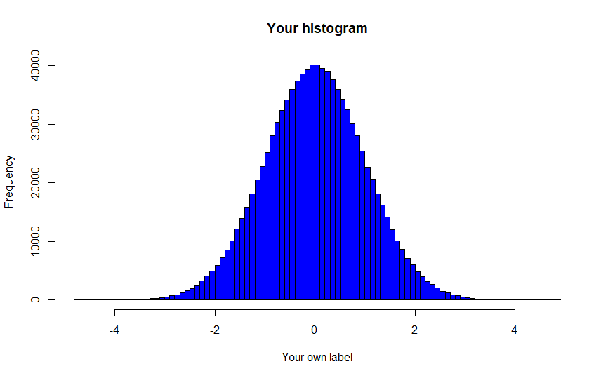
Figure 2.1: Replication Goal

Answer

# Create the histogram
a <- rnorm(1000000)
hist(a, 
     breaks=100, # set breaks to 100
     col="blue", # make bars blue
     main = "Your histogram", # Add a title
     xlab = "Your own label") # Custom label for the x-axis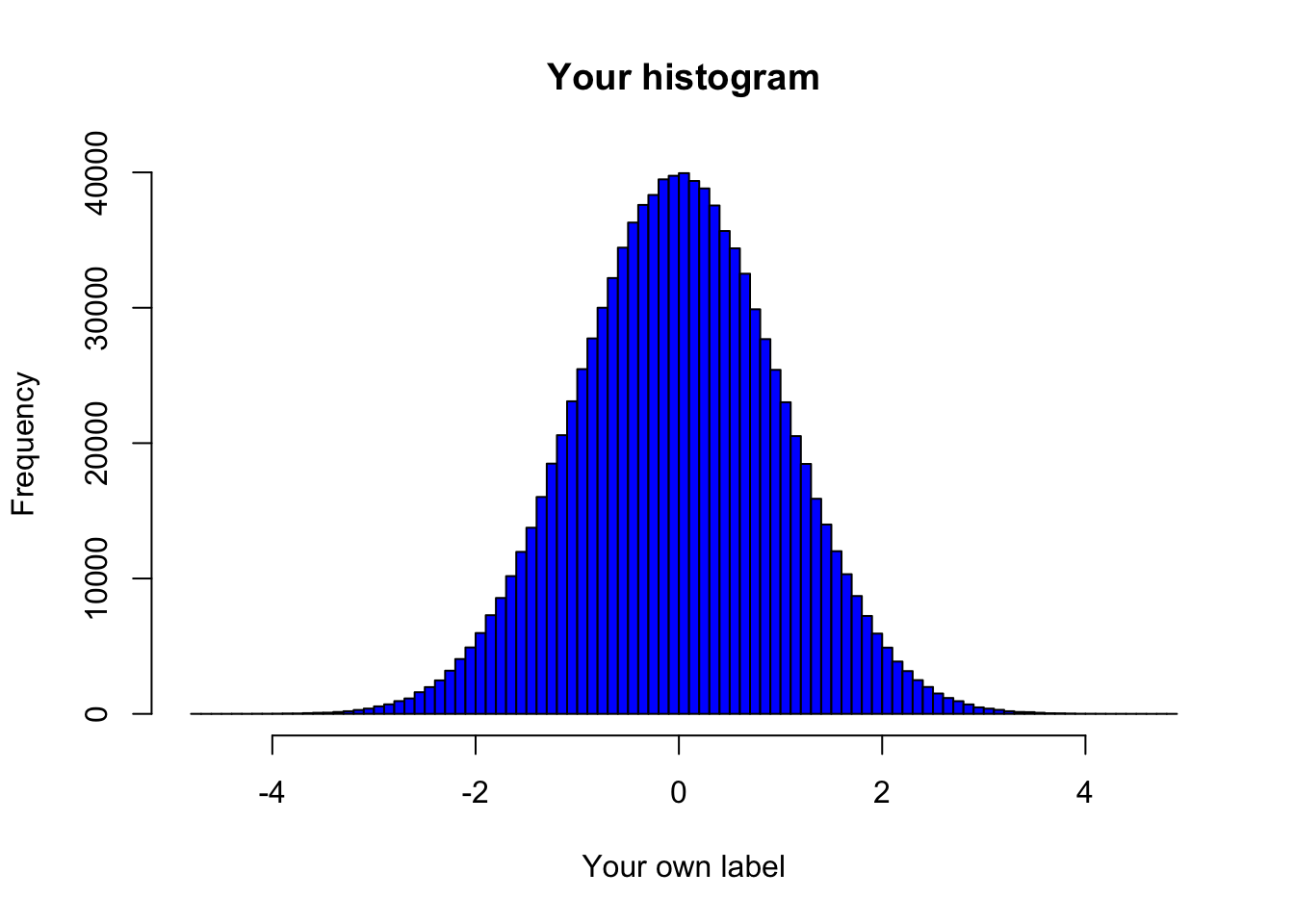


# alternative solution with nested functions
hist(rnorm(1000000), 
     breaks=100, 
     col="blue", 
     main = "Your histogram", 
     xlab = "Your own label")

2.12 Logical Operators

Logical operators are (vectors of) TRUE and FALSE statements. They are helpful for example for debugging and checking outcomes, or subsetting and manipulating data. Most importantly they are essential for programming, for example in if-statements.

When thinking about logical operators, always keep in mind that R uses recycling. So checking a condition for a vector checks each element (…and again returns a vector of the same size).

a <- c(1,5,2,7,3,9)
print(a >= 5)
#> [1] FALSE  TRUE FALSE  TRUE FALSE  TRUE

Overview of Logical Operators in R

Operator	Description
`<`	Test for less than
`<=`	Test for less than or equal to
`>`	Test for greater than
`>=`	Test for greater than or equal to
`==`	Test for equality
`!=`	Test for if not equality
`!x`	Boolean negation, for vectors
`x \| y`	Boolean x OR y, for vectors
`x & y`	Boolean x AND y, for vectors
`x \|\| y`	Boolean x OR y, for scalars
`x && y`	Boolean x AND y, for scalars
`isTRUE(x)`	Boolean test if X is TRUE, for scalars

Let’s see how logical operators work in practice:

x <- c(1,2,3)
y <- c(5,4,3)
x < y ## element-by-element comparison
#> [1]  TRUE  TRUE FALSE
x <= y
#> [1] TRUE TRUE TRUE
x > y
#> [1] FALSE FALSE FALSE
x == y
#> [1] FALSE FALSE  TRUE
x != y
#> [1]  TRUE  TRUE FALSE
mean(x) == mean(y) ## also works with results
#> [1] FALSE

Check whether a dataset has the right structure:

df <- data.frame(country=c("Germany","Austria","Germany",
                           "Austria","Austria"),
                 year=c(1990,1990,1991,1991,1991))
# Create a unique identifier
df$id <- paste0(df$country,df$year)
df[3:5,]
#>   country year          id
#> 3 Germany 1991 Germany1991
#> 4 Austria 1991 Austria1991
#> 5 Austria 1991 Austria1991
# Check: Do we have a correct panel structure?
length(unique(df$id)) == nrow(df)
#> [1] FALSE

In programming :

x <- c(3,1,4,2,5)
# In loops: We take x element by element
for (i in 1:5) {
#We test a condition and tell R what to do...
  if (x[i] >=3) print("YES!") # ...if right
  else print("NO!") #...or wrong
}
#> [1] "YES!"
#> [1] "NO!"
#> [1] "YES!"
#> [1] "NO!"
#> [1] "YES!"

For subsetting data frames, vectors, lists,…

#We can create an index vector:
x <- c(3,1,4,2,5)
index <- x >= 3
#And use it to subset x:
x[index]
#> [1] 3 4 5
#We could also keep the opposite:
x[!index]
#> [1] 1 2
#This is the same as indexing x directly:
identical(x[x>=3], x[index])
#> [1] TRUE

We can use the same logic to subset character vectors

x <- c("FC Koeln", "Hertha Berlin", "Union Berlin")
index.1 <- x == "Union Berlin" #Exactly matches
index.2 <- grepl("Berlin",x) #Partly matches

x[index.1]
#> [1] "Union Berlin"
x[index.2]
#> [1] "Hertha Berlin" "Union Berlin"

#Keep in mind that all these operators return vectors:
index.1
#> [1] FALSE FALSE  TRUE

All this works great with data frames:

df <- data.frame(
      club=c("FC Koeln", "Hertha Berlin", "Union Berlin"),
      league = c(2,1,2), stringsAsFactors = F)

league.index <- df$league == 2
club.index <- grepl("Berlin",df$club)

df[league.index & club.index, colnames(df)=="club"]
#> [1] "Union Berlin"

#We also could change this easily to end up with the FC:
df[league.index & !club.index, colnames(df)=="club"]
#> [1] "FC Koeln"

Exercise 6

Question 1: Getting to know the operators

Start by creating a vector that contains 15 draws from a random distribution (the rnorm() function helps you with this)
Run the following logical tests:
- Which elements are bigger than the mean of your vector? Store the result as an index-vector.
- How many are bigger, how many smaller?
- Subset the vector to those elements bigger than the mean. Use your index!
- Now, keep only those that are not bigger than the mean. Use your index!
- Take 15 new draws from a random distribution. Are the means the same?

Answer

# Create Vector:
vec <- rnorm(15)

# Get the mean:
mean.vec <- mean(vec)

# Which are bigger? Store the result
vec > mean.vec
#>  [1]  TRUE  TRUE  TRUE FALSE  TRUE  TRUE FALSE FALSE  TRUE
#> [10] FALSE  TRUE  TRUE FALSE FALSE  TRUE
index <- vec > mean.vec

# How many are bigger, how many smaller?
table(vec>mean.vec)
#> 
#> FALSE  TRUE 
#>     6     9
    
# Subset the vector to those elements bigger than the mean
vec[index]
#> [1] 1.3175068 1.0607302 0.6960705 1.4086656 0.5859360
#> [6] 2.0697394 0.6693823 0.9487003 0.9990897

#Now, keep only those that are *not bigger* than the mean
vec[!index]  
#> [1]  0.46737063 -0.19539254  0.02733072  0.11125477
#> [5] -0.65371958 -1.67689507

# Take 15 new draws from a random distribution. 
vec2 <- rnorm(15)

# Are the means the same?
mean.vec == mean(vec2)
#> [1] FALSE

Question 2: Logical Operators in Practice (optional)

Load some data on US states:

data(USArrests)
df <- USArrests, attach(df)

Assume you want to help Jessica Fletcher (a famous American fictional detective) find the best state to live in. Create an index for each condition and then find out which state’s the winner.
- As she wrote “murder”, not “boredom”, it should be a state with a murder rate of at least 2.
- Also, assaults should be above 70 that she has something to do in her free-time.
- However, rapes are bad. Let’s get a state with below half the average
- She likes people, but it shouldn’t be too crowded. The share of urban people should be between 50 and 70 percent.
- Which state is the winner?

Answer

  
### Question 2: Logical Operators in Practice ###   
data(USArrests)
df <- USArrests
head(df)
#>            Murder Assault UrbanPop Rape
#> Alabama      13.2     236       58 21.2
#> Alaska       10.0     263       48 44.5
#> Arizona       8.1     294       80 31.0
#> Arkansas      8.8     190       50 19.5
#> California    9.0     276       91 40.6
#> Colorado      7.9     204       78 38.7
attach(df)

# Murder-Rate above 2:
index1 <- Murder > 2

# Assaults above 70
index2 <- Assault > 70

# Rapes below half the average:
index3 <- Rape < (mean(Rape)/2)

# Urban between 50 and 70:
index4 <- UrbanPop > 50 & UrbanPop < 70

# Let's subset and find the winner:
df2 <- df[index1 & index2 & index3 & index4,]
row.names(df2)
#> [1] "Maine"

detach(df)

Appendix: A few statistical functions in R

mean(x) computes the mean
sd(x) computes the sample standard deviation
var(x) computes the sample variance
median(x) computes the media of a vector
quantile(x,probs=...) computes the supplied quantiles of a vector
summary(x) summarizes the input object (for a vector, mean, min, max, etc.)
cor(x,y) computes the correlation of two vectors
cov(x,y) computes the covariance of two vectors
Self explaining: +, -, *, /
Exponentiation: x^p, e.g. x^2 or x^10
abs(x) takes the absolute value of a vector
sqrt(x) takes the square root of a vector
log(x) takes the natural logarithm of a vector
exp(x) exponentiates the vector
min(x) returns the minimum of a vector
max(x) returns the maximum of a vector
sum(x) returns the sum of a vector
prod(x) returns the product of a vector
round(x, digits) rounds the vector to specified ## digits
trunc(x) truncates the vector to an integer
cumsum(x) returns the running sum of a vector

1 Understanding R

3 Working With Data in R