7 Statistical Models

7.1 Introduction

In this chapter, we will continue to explore the penguins dataset from the package palmerpenguins which contains size measurements for adult penguins near Palmer Station, Antarctica.

library(tidyverse)
library(palmerpenguins)

Figure 1.1: Artwork by Allison Horst

Visually, we had already stumbled upon the paradox that bill length does not seem to be positively correlated to bill depth:

# overlay scatter plot with linear model (without confidence intervals)
ggplot(penguins, aes(bill_length_mm, bill_depth_mm)) +
  geom_point() + 
  geom_smooth(method = "lm", se = FALSE)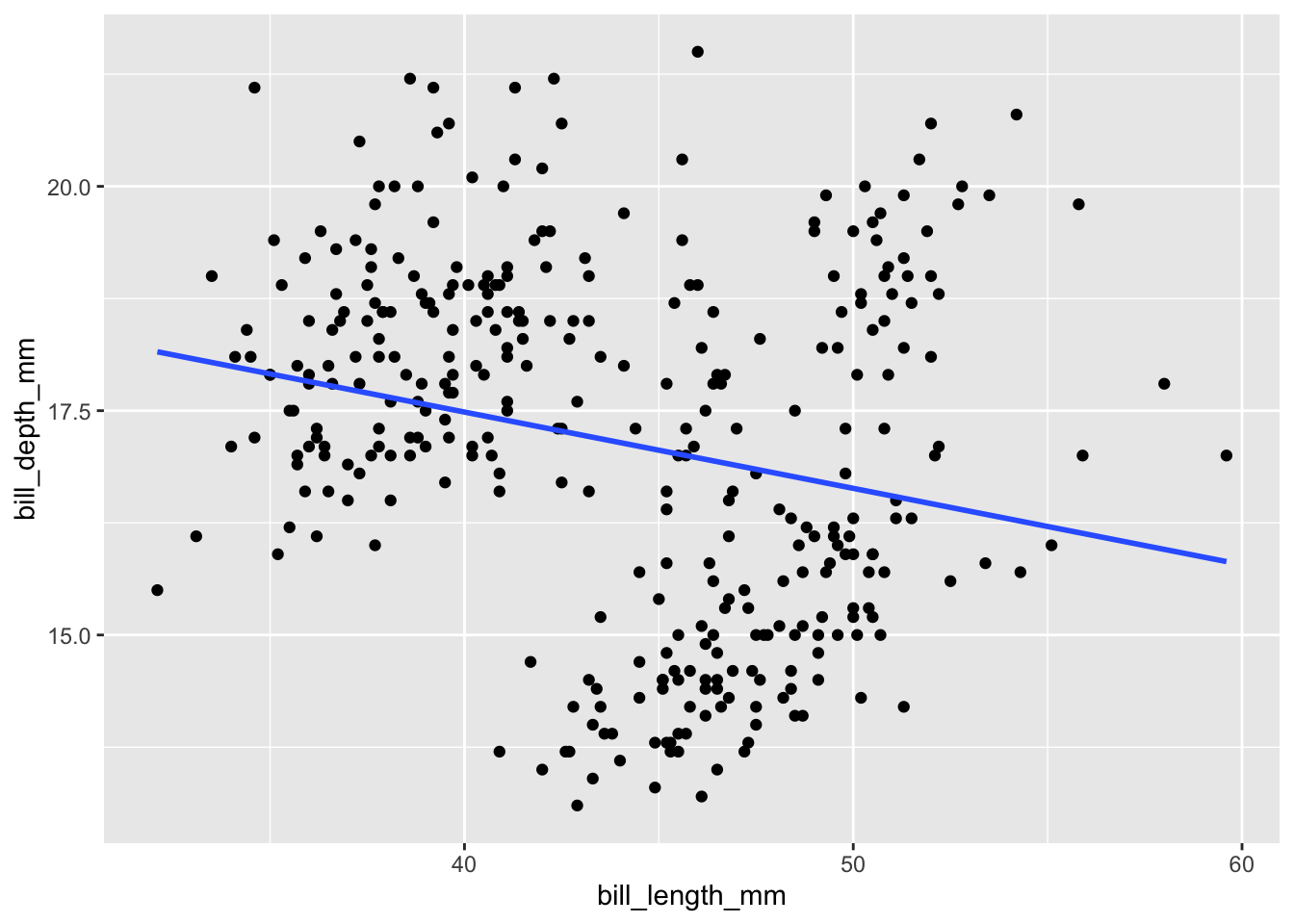

The package modelsummary (used in the chapter on data visualization to create summary statistics) confirms that the correlation coefficient between the two bill dimensions is negative for the full sample:

library(modelsummary)
datasummary_correlation(penguins)

	bill_length_mm	bill_depth_mm	flipper_length_mm	body_mass_g	year
bill_length_mm	1	.	.	.	.
bill_depth_mm	−.24	1	.	.	.
flipper_length_mm	.66	−.58	1	.	.
body_mass_g	.60	−.47	.87	1	.
year	.05	−.06	.17	.04	1

When we investigate the correlation for each penguin species, however, the negative effect vanishes (and turns positive, as expected):

ggplot(penguins, aes(bill_length_mm, bill_depth_mm, color = species)) +
  geom_point() + 
  geom_smooth(method = "lm", se = FALSE)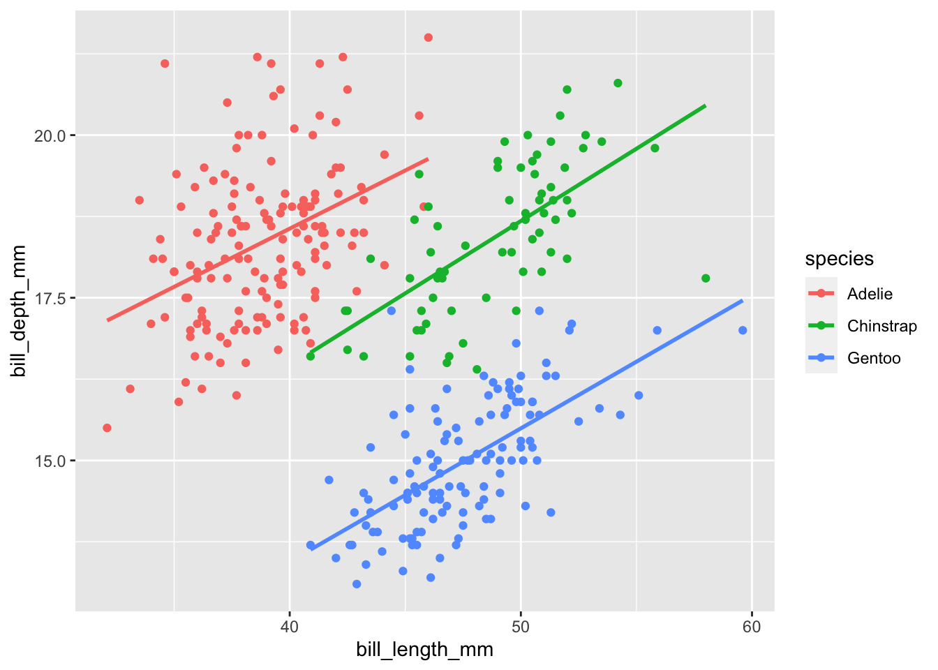

This phenomenon (an effect that vanishes or reverses when groups are combined) is an example of Simpson’s paradox. In this chapter, we will try to quantify this effect by fitting a statistical model.

7.2 Regression basics

7.2.1 Linear Regression and the model object

We can formalize the model in the context of linear regression as

\[ depth_i = \beta_0 + \beta_1 length_i + \varepsilon_i.\]

The most basic R function to fit a linear model is lm(). In fact, we have already used it implicitly when we displayed the relationship between the two variables using geom_smooth(method = "lm", se = FALSE). The following code will call the function and fit our model:

lm(bill_depth_mm ~ bill_length_mm, data = penguins)
#> 
#> Call:
#> lm(formula = bill_depth_mm ~ bill_length_mm, data = penguins)
#> 
#> Coefficients:
#>    (Intercept)  bill_length_mm  
#>       20.88547        -0.08502

The syntax is simple enough yet it deserves a few comments, especially if you are coming from single-purpose statistical software like Stata.

• The function call needs two arguments: a regression formula and the name of the dataset containing the variables.
• Dependent and independent variables are separated by the tilde sign ~.

The above call does return some output to the console (i.e., the point estimates of the two coefficients) but it behaves like any other function in R: its output is ephemeral unless you save it in a variable.

# save fitted model in a new variable
mod <- lm(bill_depth_mm ~ bill_length_mm, data = penguins)

If you have been using R for any amount of time, this will feel like second nature but if you are just coming from Stata, you might feel inclined to run something along the lines of regress bill_depth_mm bill_length_mm and expect the output to be available somewhere in the environment. What does an object that contains a statistical model even look like?

In R, most complex classes of objects are just big lists that come with custom print() and summary() functions. That way, they conceal most of their complexity while giving you nicely formatted output. We can take a look under the hood of the model object mod with

str(mod)
#> List of 13
#>  $ coefficients : Named num [1:2] 20.885 -0.085
#>   ..- attr(*, "names")= chr [1:2] "(Intercept)" "bill_length_mm"
#>  $ residuals    : Named num [1:342] 1.139 -0.127 0.541 1.535 3.056 ...
#>   ..- attr(*, "names")= chr [1:342] "1" "2" "3" "5" ...
#>  $ effects      : Named num [1:342] -317.181 -8.572 0.488 1.489 3.005 ...
#>   ..- attr(*, "names")= chr [1:342] "(Intercept)" "bill_length_mm" "" "" ...
#>  $ rank         : int 2
#>  $ fitted.values: Named num [1:342] 17.6 17.5 17.5 17.8 17.5 ...
...
# try unclass(mod) to retrieve the bare list object

As you can see, the model object contains the point estimates, residuals and fitted values as list elements. You can retrieve them using the usual $ syntax or with one of the extractor functions:

mod$coefficients
#>    (Intercept) bill_length_mm 
#>    20.88546832    -0.08502128
coef(mod)
#>    (Intercept) bill_length_mm 
#>    20.88546832    -0.08502128

Storing the fitted model in a variable allows us to re-use and modify it later and to produce nicely formatted regression output from it.

7.2.2 Formatting regression output

The most basic function that computes additional model statistics and produces formatted regression output is R’s ubiquitous summary() function.

summary(mod)
#> 
#> Call:
#> lm(formula = bill_depth_mm ~ bill_length_mm, data = penguins)
#> 
#> Residuals:
#>     Min      1Q  Median      3Q     Max 
#> -4.1381 -1.4263  0.0164  1.3841  4.5255 
#> 
#> Coefficients:
#>                Estimate Std. Error t value Pr(>|t|)    
#> (Intercept)    20.88547    0.84388  24.749  < 2e-16 ***
#> bill_length_mm -0.08502    0.01907  -4.459 1.12e-05 ***
#> ---
#> Signif. codes:  
#> 0 '***' 0.001 '**' 0.01 '*' 0.05 '.' 0.1 ' ' 1
#> 
#> Residual standard error: 1.922 on 340 degrees of freedom
#>   (2 observations deleted due to missingness)
#> Multiple R-squared:  0.05525,    Adjusted R-squared:  0.05247 
#> F-statistic: 19.88 on 1 and 340 DF,  p-value: 1.12e-05

There are more modern tools to format regression output, however. The first one is broom::tidy(), which arranges basic model statistics from a variety of different model classes in a tibble. This format certainly does not give you publication-ready tables but it is ideal for processing the data further.

broom::tidy(mod)
#> # A tibble: 2 × 5
#>   term           estimate std.error statistic  p.value
#>   <chr>             <dbl>     <dbl>     <dbl>    <dbl>
#> 1 (Intercept)     20.9       0.844      24.7  4.72e-78
#> 2 bill_length_mm  -0.0850    0.0191     -4.46 1.12e- 5

The second one is modelsummary::modelsummary(), which takes this output a step further and produces nice-looking tables in various formats (Markdown, PDF, HTML…). Inside of a dynamic document (like this one), the HTML output is automatically embedded:

modelsummary(mod)

	(1)
(Intercept)	20.885
	(0.844)
bill_length_mm	−0.085
	(0.019)
Num.Obs.	342
R2	0.055
R2 Adj.	0.052
AIC	1421.6
BIC	1433.1
Log.Lik.	−707.776
F	19.884
RMSE	1.92

The documentation is excellent so you will be asked to figure out the most important formatting options yourself in the exercises. To avoid major accidents, these are the two biggest caveats for economists:

1. By default, no significance stars will be shown in the regression output. If you enable them with stars = TRUE, modelsummary() will stick to R’s notation that uses stricter confidence levels. Provide a named vector instead to get the notation common in the economics literature: stars = c("***" = 0.01, "**" = 0.05, "*" = 0.1)
2. In reality, you will almost never want to use the default standard errors. Provide a vcov argument to specify robust or clustered standard errors.

7.2.3 Exercises

7.2.3.1 Question 1

Split the penguins dataset into three according to species and fit a linear model (bill_depth_mm ~ bill_length_mm) on each dataset. Display the regression output from all three models as columns of a single table using modelsummary().

Answer

Apart from the modelsummary() function, all operations should be familiar to you by now so we only add short comments in the code. modelsummary() takes a single model object or a list of model objects as the first argument. That means you cannot call modelsummary(mod1, mod2, mod3) directly. In the code below, map() returns a list of models that we can pass as a single argument to produce formatted regression output. Note that map() preserves the names of the list elements from penguins_split which allows modelsummary() to use them as column headings.

# split data
adelie <- penguins %>% filter(species == "Adelie")
chinstrap <- penguins %>% filter(species == "Chinstrap")
gentoo <- penguins %>% filter(species == "Gentoo")

# bind as named list
penguins_split <- list("Adelie" = adelie, 
                       "Chinstrap" = chinstrap, 
                       "Gentoo" = gentoo)

# fit model on each element of the list
mod_split <- map(penguins_split, ~lm(bill_depth_mm ~ bill_length_mm, data = .x))

# format regression output
modelsummary(mod_split)

	Adelie	Chinstrap	Gentoo
(Intercept)	11.409	7.569	5.251
	(1.339)	(1.551)	(1.055)
bill_length_mm	0.179	0.222	0.205
	(0.034)	(0.032)	(0.022)
Num.Obs.	151	68	123
R2	0.153	0.427	0.414
R2 Adj.	0.148	0.418	0.409
AIC	467.6	177.4	283.7
BIC	476.7	184.0	292.1
Log.Lik.	−230.808	−85.679	−138.834
RMSE	1.12	0.85	0.75

The solution above uses only basic tidyverse functions that you have encountered before. We can streamline the code by using the function split() to split the dataset based on the species and use their names for each resulting dataset:

# create list of dataframes according to species
penguin_species <- penguins |> 
  split(~species)

# apply regression to each list element and display
penguin_species |> 
  map(\(df) lm(bill_depth_mm ~ bill_length_mm, data = df)) |> 
  modelsummary::modelsummary()

	Adelie	Chinstrap	Gentoo
(Intercept)	11.409	7.569	5.251
	(1.339)	(1.551)	(1.055)
bill_length_mm	0.179	0.222	0.205
	(0.034)	(0.032)	(0.022)
Num.Obs.	151	68	123
R2	0.153	0.427	0.414
R2 Adj.	0.148	0.418	0.409
AIC	467.6	177.4	283.7
BIC	476.7	184.0	292.1
Log.Lik.	−230.808	−85.679	−138.834
RMSE	1.12	0.85	0.75

An even more concise solution can be achieved with the package fixest that we introduce below.

7.2.3.2 Question 2

It was mentioned above that you need to manually tweak the significance stars notation to match the economist default like so:

modelsummary(mod, stars = c("***" = 0.01, "**" = 0.05, "*" = 0.1))

Write a custom function called modsum() that behaves the same way as modelsummary() but adds significance stars like an economist would.

Answer

modsum <- function(...) {
  modelsummary(..., stars = c("***" = 0.01, "**" = 0.05, "*" = 0.1))
}

Don’t worry if you used an argument name (such as x) instead of the dots – your function will do what was asked in the question. The dots allow you pass an unspecified number of arguments to the function without having to name each argument in the function definition. That way, you could pass another argument (e.g., vcov = "robust") to modelsummary() which would not be possible otherwise.

7.2.3.3 Question 3

Read the help file of modelsummary() to make your regression output from the first exercise more beautiful. It should resemble the following output:

Table 7.1: Correlation between bill length and bill depth

	Adelie	Chinstrap	Gentoo
Bill length (mm)	0.179***	0.222***	0.205***
	(0.034)	(0.032)	(0.022)
Num.Obs.	151	68	123
R2 Adj.	0.148	0.418	0.409
* p < 0.1, ** p < 0.05, *** p < 0.01

Useful function arguments include stars, coef_omit, coef_rename, gof_omit and title.

Answer

There are many ways to get the output from above. Basically, modelsummary() allows you to provide a “positive list” of coefficients and goodness-of-fit (“gof”) statistics to include with the *_map argument; or a “negative list” of entries to exclude with *_omit.

modelsummary(mod_split, 
             stars = c("***" = 0.01, "**" = 0.05, "*" = 0.1),
             coef_omit = "Int",
             coef_rename = c(bill_length_mm = "Bill length (mm)"),
             gof_omit = "IC$|Lik.|RMSE|R2$", 
             title = "Correlation between bill length and bill depth")

This is the point where Stata users will start missing variable labels. They are not implemented in base R but there are many workarounds. First, note that you can have non-syntactic variable names (e.g., including spaces) if you put backticks around them. So `Bill length (mm)` would be a perfectly valid variable name that would appear without backticks in the regression output.

Second, there are multiple packages that implement variable labels in R. In fact, in R you can specify any number of attributes (such as labels) to any object. When you import a .dta file with the haven package, it will preserve Stata’s variable labels by default. To see them, open the dataset in the R Studio viewer.

The most natural way in R, however, is to save the variable names and their labels as a named vector so you can re-use them later.

dict <- c(bill_length_mm = "Bill length (mm)")

modelsummary(mod_split,
             coef_map = dict,
             gof_map = NA)

	Adelie	Chinstrap	Gentoo
Bill length (mm)	0.179	0.222	0.205
	(0.034)	(0.032)	(0.022)

Note that while the *_omit arguments accept regular expressions matching the name as displayed in the regression output, the *_map arguments always refer to “raw” names. For coefficients, this means the variable names in the dataset; for goodness-of-fit statistics this refers to the following list:

modelsummary::gof_map
#>                          raw              clean fmt  omit
#> 1                       nobs           Num.Obs.   0 FALSE
#> 2                       nimp           Num.Imp.   0 FALSE
#> 3                  nclusters         Num.Clust.   0 FALSE
#> 4                    nblocks         Num.Blocks   0 FALSE
#> 5                  r.squared                 R2   3 FALSE
#> 6                         r2                 R2   3 FALSE
#> 7              adj.r.squared            R2 Adj.   3 FALSE
#> 8                r2.adjusted            R2 Adj.   3 FALSE
...

So if we only wanted to include the adjusted R squared and the number of observations, the following code would work:

modelsummary(mod_split,
             coef_map = dict,
             gof_map = c("adj.r.squared", "nobs"))

	Adelie	Chinstrap	Gentoo
Bill length (mm)	0.179	0.222	0.205
	(0.034)	(0.032)	(0.022)
R2 Adj.	0.148	0.418	0.409
Num.Obs.	151	68	123

7.2.3.4 Question 4

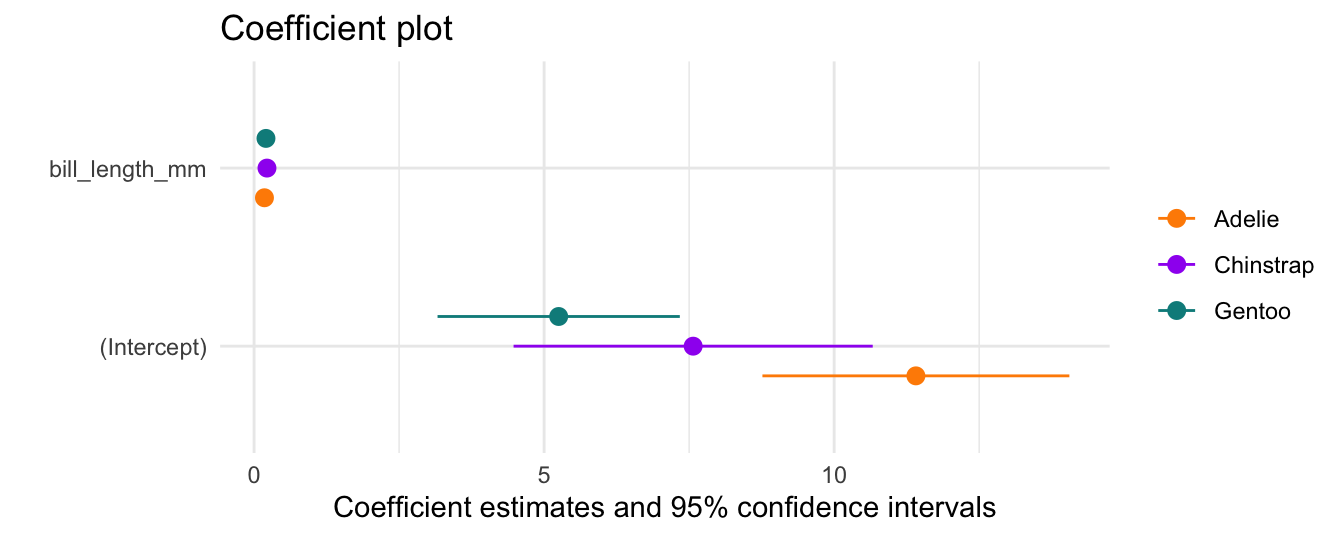
Display your regression results from the first exercise as a coefficient plot with modelsummary::modelplot(). This is actually a ggplot! Use your knowledge from the chapter on data visualization to add a title (“Coefficient plot”) and adjust the colors: values = c("darkorange","purple","cyan4").

Answer

modelplot(mod_split) + 
  labs(title = "Coefficient plot") +
  scale_color_manual(values = c("darkorange","purple","cyan4"))

Note that the variation of the point estimate for the intercept is much larger (in absolute terms) than that of bill_length_mm, the variable we are interested in. To emphasize its variation, we could either remove the intercept from the plot or scale each variable by its standard deviation. The argument to hide variables from the output is standardized across the modelsummary package, so coef_omit works just fine in this coefficient plot.

7.3 Modifying formula objects

In our call to lm() we typed out the regression formula, yet it is often advantageous to store the formula in a separate object. That way we can build upon an existing formula should we decide to modify our econometric specification later on. As always in programming, removing redundancy lowers the chance of making mistakes and makes it easier to keep code up to date.

The code chunk below presents an alternative way to fit our linear model from above. Note that the formula is not a character string and therefore does not need quotation marks. You can think of it as a piece of raw code with variable names as placeholders for actual data. R will evaluate the code when you specify which dataset the variable names refer to in the call to lm().

# store formula
f <- bill_depth_mm ~ bill_length_mm

# fit model using the formula object
lm(f, data = penguins)

Of course, the formula syntax allows us to implement common econometric specifications, such as multiple explanatory variables, dummy variables, interaction terms, non-linear relationships and so on.

To add an explanatory variable (e.g., species), simply append it to the formula with a plus sign. Note that species is a categorical variable with three levels. Unlike Stata, R is smart enough to create dummy variables for each level automatically:

# add variable species as regressor
lm(bill_depth_mm ~ bill_length_mm + species, data = penguins)
#> 
#> Call:
#> lm(formula = bill_depth_mm ~ bill_length_mm + species, data = penguins)
#> 
#> Coefficients:
#>      (Intercept)    bill_length_mm  speciesChinstrap  
#>          10.5922            0.1999           -1.9332  
#>    speciesGentoo  
#>          -5.1060

In the example above, one level is dropped because an intercept is included in the formula by default. To remove it, add +0 or -1 to your formula:

# remove intercept
lm(bill_depth_mm ~ bill_length_mm + species + 0, data = penguins)
#> 
#> Call:
#> lm(formula = bill_depth_mm ~ bill_length_mm + species + 0, data = penguins)
#> 
#> Coefficients:
#>   bill_length_mm     speciesAdelie  speciesChinstrap  
#>           0.1999           10.5922            8.6590  
#>    speciesGentoo  
#>           5.4862

To specify an interaction effect, R uses the multiplication sign *. This intuitive notation includes both main effects by default, which is often what we want. To omit the main effects, use : instead:

# interaction with main effects
lm(bill_depth_mm ~ bill_length_mm*body_mass_g, data = penguins)
#> 
#> Call:
#> lm(formula = bill_depth_mm ~ bill_length_mm * body_mass_g, data = penguins)
#> 
#> Coefficients:
#>                (Intercept)              bill_length_mm  
#>                 14.1188169                   0.1822208  
#>                body_mass_g  bill_length_mm:body_mass_g  
#>                  0.0006073                  -0.0000402

# interaction without main effects
lm(bill_depth_mm ~ bill_length_mm:body_mass_g, data = penguins)
#> 
#> Call:
#> lm(formula = bill_depth_mm ~ bill_length_mm:body_mass_g, data = penguins)
#> 
#> Coefficients:
#>                (Intercept)  bill_length_mm:body_mass_g  
#>                  2.017e+01                  -1.613e-05

A Stata dataset that has been prepared for statistical analysis often contains hundreds of variables, each reflecting a certain transformation (such as the logarithm). In R, this is usually not necessary because you can transform variables on the fly, within the formula. For example, to investigate elasticities there is no need to create new variables – simply wrap the variable name inside log():

# transform variables on the fly
lm(log(bill_depth_mm) ~ log(bill_length_mm), data = penguins)
#> 
#> Call:
#> lm(formula = log(bill_depth_mm) ~ log(bill_length_mm), data = penguins)
#> 
#> Coefficients:
#>         (Intercept)  log(bill_length_mm)  
#>              3.7344              -0.2382

The greatest feature of formula and model objects is that you can modify them later on. This allows you to define a base specification that is common to all your models and gradually extend it by adding variables. The function to modify existing formula objects is update(). It takes the existing formula as the first argument and modifies it as specified in the second argument which is a (partial) redefinition of the formula.

You can either replace the left-hand side or the right-hand side of the formula by writing new variable names before and after the tilde sign or you can add variables to each side. Use a dot as a placeholder to preserve the variables that are already in the formula and add or remove variables with plus and minus.

f
#> bill_depth_mm ~ bill_length_mm
update(f, . ~ sex) # replace RHS
#> bill_depth_mm ~ sex
update(f, body_mass_g ~ .) # replace LHS
#> body_mass_g ~ bill_length_mm
update(f, ~ . + sex) # add predictor
#> bill_depth_mm ~ bill_length_mm + sex
update(f, ~ . - bill_length_mm) # remove a predictor
#> bill_depth_mm ~ 1

If you have already fit a model, you can use update() to modify the model object directly. This works because the model object (a big list, as we had seen) is aware of the formula it is based on.

mod
#> 
#> Call:
#> lm(formula = bill_depth_mm ~ bill_length_mm, data = penguins)
#> 
#> Coefficients:
#>    (Intercept)  bill_length_mm  
#>       20.88547        -0.08502

# update formula
update(mod, . ~ . + sex)
#> 
#> Call:
#> lm(formula = bill_depth_mm ~ bill_length_mm + sex, data = penguins)
#> 
#> Coefficients:
#>    (Intercept)  bill_length_mm         sexmale  
#>        22.5614         -0.1458          2.0133

In addition to changing the underlying formula of a model object, you can also exchange the dataset on which it was fit. The following code chunk applies the existing regression formula to a subset of the penguins dataset that contains only Adelie penguins.

# update data
adelie <- penguins %>% filter(species == "Adelie")
update(mod, data = adelie)
#> 
#> Call:
#> lm(formula = bill_depth_mm ~ bill_length_mm, data = adelie)
#> 
#> Coefficients:
#>    (Intercept)  bill_length_mm  
#>        11.4091          0.1788

7.3.1 Exercises

7.3.1.1 Question 1

Let f <- bill_depth_mm ~ bill_length_mm be our base specification. Use update() to create two new formula objects based on f, one that additionally includes body_mass_g and one that additionally includes body_mass_g and its interaction with bill_length_mm. Bind all three models into a list and fit a linear model on each one. Display your results side-by-side with modelsummary().

Answer

Apart from updating the formula object, this exercise is similar to a previous one. Note that here we are using map() to apply multiple formulas to the same dataset whereas above we used it to apply the same formula to multiple datasets.

# define base formula
f <- bill_depth_mm ~ bill_length_mm

# create list with updated formulas
fmls <- list(f,
             update(f, ~ . + body_mass_g),
             update(f, ~ . + body_mass_g + body_mass_g:bill_length_mm))

# fit models and view as regression table
fmls |> 
  map(\(f) lm(f, data = penguins)) |> 
  modelsummary(gof_map = NA)

	(1)	(2)	(3)
(Intercept)	20.885	21.344	14.119
	(0.844)	(0.767)	(4.370)
bill_length_mm	−0.085	0.026	0.182
	(0.019)	(0.022)	(0.096)
body_mass_g		−0.001	0.001
		(0.000)	(0.001)
bill_length_mm × body_mass_g			0.000
			(0.000)

7.3.1.2 Question 2

Write a formula to regress bill_depth_mm on the sum of bill_length_mm and flipper_length_mm. What is the problem when you try to compute the sum on the fly, within the formula? Read the formula help file ?formula and find out how to solve it.

Answer

The plus sign has a special meaning within a formula: it adds explanatory variables to a model. To use it in its arithmetic sense, we have to protect it by wrapping it inside of I():

lm(bill_depth_mm ~ I(bill_length_mm + flipper_length_mm), data = penguins)
#> 
#> Call:
#> lm(formula = bill_depth_mm ~ I(bill_length_mm + flipper_length_mm), 
#>     data = penguins)
#> 
#> Coefficients:
#>                           (Intercept)  
#>                              31.13272  
#> I(bill_length_mm + flipper_length_mm)  
#>                              -0.05711

Note that ^ has a special meaning inside of formulas as well which means that we have to write I(x^2) to create a squared term. To create higher-order polynomials, have a look at the poly() function.

7.3.1.3 Question 3

We now want to include dummy variables for each year to remove fluctuations over time. What is the problem in the code below and how do we fix it?

lm(bill_depth_mm ~ 0 + bill_length_mm + year, data = penguins)
#> 
#> Call:
#> lm(formula = bill_depth_mm ~ 0 + bill_length_mm + year, data = penguins)
#> 
#> Coefficients:
#> bill_length_mm            year  
#>       -0.08504         0.01040

Answer

In the penguins dataset, the variable type of year is numeric, not categorical. A quick and dirty fix is to convert it to a categorical (= factor) variable:

lm(bill_depth_mm ~ 0 + bill_length_mm + factor(year), data = penguins)
#> 
#> Call:
#> lm(formula = bill_depth_mm ~ 0 + bill_length_mm + factor(year), 
#>     data = penguins)
#> 
#> Coefficients:
#>   bill_length_mm  factor(year)2007  factor(year)2008  
#>         -0.08579          21.17989          20.64932  
#> factor(year)2009  
#>         20.93871

7.4 Panel data and the fixest package

Panel data consists of repeated cross sections. Usually, that means we can observe different entities (e.g., countries) over time. As an example of panel data we will use the trade dataset that comes with the fixest package. It contains information on the trade of different products between members of the European Union (EU15) as reported by Eurostat.

library(fixest)
as_tibble(trade)
#> # A tibble: 38,325 × 6
#>    Destination Origin Product  Year dist_km    Euros
#>    <fct>       <fct>    <int> <dbl>   <dbl>    <dbl>
#>  1 LU          BE           1  2007    140.  2966697
#>  2 BE          LU           1  2007    140.  6755030
#>  3 LU          BE           2  2007    140. 57078782
#>  4 BE          LU           2  2007    140.  7117406
#>  5 LU          BE           3  2007    140. 17379821
#>  6 BE          LU           3  2007    140.  2622254
#>  7 LU          BE           4  2007    140. 64867588
#>  8 BE          LU           4  2007    140. 10731757
#>  9 LU          BE           5  2007    140.   330702
#> 10 BE          LU           5  2007    140.     7706
#> # ℹ 38,315 more rows

We do not have to treat panel data any differently than cross-sectional data but we will forgo the opportunity to exploit the panel structure. If we wanted to investigate how the distance between two countries affects the trade between them, we could fit a linear model just as before. This estimation is called “pooled OLS” (ordinary least squares) because we are treating each observation of the trade value the same, irrespective of the associated country pair or product category. Don’t be irritated by the special name though: the way we fit our linear model remains exactly the same.

lm(log(Euros) ~ log(dist_km), data = trade)
#> 
#> Call:
#> lm(formula = log(Euros) ~ log(dist_km), data = trade)
#> 
#> Coefficients:
#>  (Intercept)  log(dist_km)  
#>        28.32         -1.91

So what is special about panel data? We can exploit the panel structure to remove some unwanted (and potentially unobserved) confounding factors that are either specific to an entity and constant over time (e.g., cultural factors in a given country) or specific to a point in time and the same for all entities (e.g., a shock to the world economy in a given year). To remove these confounding factors, we include dummy variables for each entity or each point in time. These dummy variables are referred to as fixed effects.

Of course, you can include these dummy variables manually. In fact we already did so when we added species as a regressor to analyze the penguins dataset. In practice, however, manually adding fixed effects is not a good idea. First, because it is computationally inefficient; second, because our regression output will be cluttered up by the estimated coefficients of each dummy variable.

To perform fast fixed effect regressions, we will use the package fixest. This package has emerged as the fastest and most comprehensive R package to analyze panel data. As such, it has replaced the former go-to solution, the package plm. It is still under active development, so feel free to download the development versions or file bug reports on its GitHub repository. Stata users will rejoice: the package design is somewhat inspired by Stata functionality and conversion cheat-sheets (like this one or this one) make the transition easy.

The function feols (think: fixed-effects OLS) is a replacement for our tried and trusted lm() function. It augments the formula syntax that was introduced above to accommodate fixed effects and even notation for instrumental variable (IV) estimations. Make sure to stick to this order (fixed effects, then IV notation) and separate the elements with the pipe symbol | within a formula:

# pooled OLS (equivalent to lm)
feols(log(Euros) ~ log(dist_km), data = trade)
#> OLS estimation, Dep. Var.: log(Euros)
#> Observations: 38,325 
#> Standard-errors: IID 
#>              Estimate Std. Error  t value  Pr(>|t|)    
#> (Intercept)  28.32169   0.169621 166.9702 < 2.2e-16 ***
#> log(dist_km) -1.90965   0.024009 -79.5379 < 2.2e-16 ***
#> ---
#> Signif. codes:  0 '***' 0.001 '**' 0.01 '*' 0.05 '.' 0.1 ' ' 1
#> RMSE: 2.97663   Adj. R2: 0.141666

# fixed effects for product categories
feols(log(Euros) ~ log(dist_km) | Product, data = trade)
#> OLS estimation, Dep. Var.: log(Euros)
#> Observations: 38,325 
#> Fixed-effects: Product: 20
#> Standard-errors: Clustered (Product) 
#>              Estimate Std. Error  t value  Pr(>|t|)    
#> log(dist_km) -1.99758   0.075647 -26.4066 < 2.2e-16 ***
#> ---
#> Signif. codes:  0 '***' 0.001 '**' 0.01 '*' 0.05 '.' 0.1 ' ' 1
#> RMSE: 2.68883     Adj. R2: 0.299274
#>                 Within R2: 0.180891

# add multiple fixed effects with +; specify FE interactions with ^
feols(log(Euros) ~ log(dist_km) | Product + Destination + Origin, data = trade)
#> OLS estimation, Dep. Var.: log(Euros)
#> Observations: 38,325 
#> Fixed-effects: Product: 20,  Destination: 15,  Origin: 15
#> Standard-errors: Clustered (Product) 
#>              Estimate Std. Error  t value  Pr(>|t|)    
#> log(dist_km) -2.16893   0.076932 -28.1928 < 2.2e-16 ***
#> ---
#> Signif. codes:  0 '***' 0.001 '**' 0.01 '*' 0.05 '.' 0.1 ' ' 1
#> RMSE: 1.74798     Adj. R2: 0.703647
#>                 Within R2: 0.218273

Performing IV regressions is beyond the scope of this course so we will not discuss its notation here. A good place to read up on this topic is the corresponding chapter of the fixest walkthrough. We will, however, have a look at the syntactic sugar of the augmented formula notation that makes our economist lives much more convenient.

Switching back to the penguins dataset, let’s assume we not only want to explain flipper length but also bill length with the penguin’s weight. Instead of fitting two separate models, we can simply insert a vector of variable names into the formula:

feols(c(flipper_length_mm, bill_length_mm) ~ body_mass_g, data = penguins)
#> Standard-errors: IID 
#> Dep. var.: flipper_length_mm
#>               Estimate Std. Error t value  Pr(>|t|)    
#> (Intercept) 136.729559   1.996835 68.4731 < 2.2e-16 ***
#> body_mass_g   0.015276   0.000467 32.7222 < 2.2e-16 ***
#> ---
#> Dep. var.: bill_length_mm
#>              Estimate Std. Error t value  Pr(>|t|)    
#> (Intercept) 26.898872   1.269148 21.1944 < 2.2e-16 ***
#> body_mass_g  0.004051   0.000297 13.6544 < 2.2e-16 ***

To make the call even more concise (but less specific), we can even use a regular expression instead of the variable names:

feols(..("length") ~ body_mass_g, data = penguins)
#> Standard-errors: IID 
#> Dep. var.: bill_length_mm
#>              Estimate Std. Error t value  Pr(>|t|)    
#> (Intercept) 26.898872   1.269148 21.1944 < 2.2e-16 ***
#> body_mass_g  0.004051   0.000297 13.6544 < 2.2e-16 ***
#> ---
#> Dep. var.: flipper_length_mm
#>               Estimate Std. Error t value  Pr(>|t|)    
#> (Intercept) 136.729559   1.996835 68.4731 < 2.2e-16 ***
#> body_mass_g   0.015276   0.000467 32.7222 < 2.2e-16 ***

What works on the left-hand side of the formula also works on the right-hand side. The syntax, however, is slightly different: we can wrap the variable names inside of sw() (“step wise”) or csw() (“cumulative step wise”) instead of c() to introduce additional explanatory variables to the model one by one, as is often the case in regression output.

feols(flipper_length_mm ~ csw(bill_depth_mm, body_mass_g, sex), data = penguins)
#> Standard-errors: IID 
#> Expl. vars.: bill_depth_mm
#>                Estimate Std. Error  t value  Pr(>|t|)    
#> (Intercept)   272.21899   5.412576  50.2938 < 2.2e-16 ***
#> bill_depth_mm  -4.15737   0.313515 -13.2605 < 2.2e-16 ***
#> ---
#> Expl. vars.: bill_depth_mm + body_mass_g
#>                 Estimate Std. Error  t value   Pr(>|t|)    
#> (Intercept)   171.592099   4.721393 36.34353  < 2.2e-16 ***
#> bill_depth_mm  -1.582219   0.197458 -8.01294 1.8231e-14 ***
#> body_mass_g     0.013437   0.000486 27.63528  < 2.2e-16 ***
#> ---
#> Expl. vars.: bill_depth_mm + body_mass_g + sex
#>                 Estimate Std. Error   t value   Pr(>|t|)
#> (Intercept)   172.605600   7.082544 24.370565  < 2.2e-16
#> bill_depth_mm  -1.602590   0.287894 -5.566595 5.3970e-08
#> body_mass_g     0.013226   0.000722 18.323764  < 2.2e-16
#> sexmale         0.452492   1.102675  0.410358 6.8181e-01
#>                  
#> (Intercept)   ***
#> bill_depth_mm ***
#> body_mass_g   ***
#> sexmale

To produce formatted regression output, modelsummary() works just fine. The fixest package design is a bit idiosyncratic though, so advanced features may only be accessible through fixest::summary.fixest() and fixest::etable(), two functions provided by the package creators.

As a final note: fixest is not limited to linear regression using the feols() function. Additional functions like feglm(), fepois() and fenegbin() extend fixed effects and IV support to a variety of other model classes such as logit, probit, Poisson, negative binomial, and so on.

7.4.1 Exercises

7.4.1.1 Question 1

Open the help file to figure out how to make our regression from earlier on each subset of penguins much easier with feols(). Our goal was to estimate the equation bill_depth_mm ~ bill_length_mm for each penguin species separately.

Answer

fixest::feols(bill_depth_mm ~ bill_length_mm,
              data = penguins, 
              split = ~species) %>% 
  modelsummary()

	sample: Adelie	sample: Chinstrap	sample: Gentoo
(Intercept)	11.409	7.569	5.251
	(1.339)	(1.551)	(1.055)
bill_length_mm	0.179	0.222	0.205
	(0.034)	(0.032)	(0.022)
Num.Obs.	151	68	123
R2	0.153	0.427	0.414
R2 Adj.	0.148	0.418	0.409
AIC	465.6	175.4	281.7
BIC	471.7	179.8	287.3
RMSE	1.12	0.85	0.75
Std.Errors	IID	IID	IID

7.4.1.2 Question 2

Create the regression output below with a single call to feols() and modelsummary():

	lhs: flipper_length_mm; rhs: bill_depth_mm	lhs: flipper_length_mm; rhs: bill_depth_mm + body_mass_g	lhs: bill_length_mm; rhs: bill_depth_mm	lhs: bill_length_mm; rhs: bill_depth_mm + body_mass_g
bill_depth_mm	−4.157***	−1.582***	−0.650***	0.163
	(0.314)	(0.197)	(0.146)	(0.137)
body_mass_g		0.013***		0.004***
		(0.000)		(0.000)
Num.Obs.	342	342	342	342
R2 Adj.	0.339	0.796	0.052	0.353
* p < 0.1, ** p < 0.05, *** p < 0.01

Answer

Each column in the table represents a different combination of the dependent variable and explanatory variables. To introduce both explanatory variables for each dependent variable step by step, use the csw() function on the right-hand side and concatenate the dependent variables as a vector on the left-hand side. Take care not to use the plus sign to add variables though! Our variables are function arguments now, and the formula syntax does not work within c() or csw().

feols(c(flipper_length_mm, bill_length_mm) ~ csw(bill_depth_mm, body_mass_g),
      data = penguins) %>%
  modelsummary(
    stars = c("***" = 0.01, "**" = 0.05, "*" = 0.1),
    coef_omit = "Int",
    gof_map = c("nobs", "adj.r.squared")
  )

7.4.1.3 Question 3

Use countrycode::countrycode() to add a dummy variable to the trade dataset that equals one for trade flows between countries that use the same currency and zero otherwise. The country codes given in the data are 2-character ISO codes, known by countrycode() as "iso2c". Save your dataset and have a look at the distribution of the new variable.

Hint: If your Help pane is wide enough, there is a second search box below the global search that allows you to search for “currency” within the help file for countrycode().

# preview as tibble (better formatting)
as_tibble(trade)
#> # A tibble: 38,325 × 6
#>    Destination Origin Product  Year dist_km    Euros
#>    <fct>       <fct>    <int> <dbl>   <dbl>    <dbl>
#>  1 LU          BE           1  2007    140.  2966697
#>  2 BE          LU           1  2007    140.  6755030
#>  3 LU          BE           2  2007    140. 57078782
#>  4 BE          LU           2  2007    140.  7117406
#>  5 LU          BE           3  2007    140. 17379821
#>  6 BE          LU           3  2007    140.  2622254
#>  7 LU          BE           4  2007    140. 64867588
#>  8 BE          LU           4  2007    140. 10731757
#>  9 LU          BE           5  2007    140.   330702
#> 10 BE          LU           5  2007    140.     7706
#> # ℹ 38,315 more rows

Answer

This question is of course not more than a shameless plug to introduce you to the countrycode package. It is indispensable to harmonize your country identifiers before merging datasets. Not only does it allow you to translate between ISO codes, country names, Correlates of War and Polity IV identifiers, it can also return the continent a country belongs to, the currency and even the country’s emoji flag!

library(countrycode)

countrycode(
  c("DEU", "FRA", "CHN"),
  "iso3c",
  "unicode.symbol"
)
#> [1] "🇩🇪" "🇫🇷" "🇨🇳"

In our example, the destination format is "currency":

# create new variables
trade_currency <- trade %>% 
  as_tibble() %>% 
  mutate(
    currency_dest = countrycode::countrycode(Destination, "iso2c", "currency"),
    currency_orig = countrycode::countrycode(Origin, "iso2c", "currency")
    ) %>% 
  mutate(same_currency = (currency_dest == currency_orig))

# view distribution
trade_currency %>% 
  count(same_currency)
#> # A tibble: 2 × 2
#>   same_currency     n
#>   <lgl>         <int>
#> 1 FALSE         14702
#> 2 TRUE          23623

7.4.1.4 Question 4

The model below uses the dataset from the previous question. Update the model object below to replace Origin and Destination fixed effects with fixed effects for each level of the dummy variable you created earlier. This allows us to remove the effect of sharing a currency from the effect of distance on trade. You will need to use the pipe symbol | to separate fixed effects from other explanatory variables.

mod_currency <- feols(log(Euros) ~ log(dist_km) | Origin + Destination, data = trade_currency)

Answer

The syntax for update() does not change much but we now have a third “slot” for fixed effects that is separated from other explanatory variables. Since we do not write a dot after the pipe symbol, our new fixed effects replace the old ones.

update(mod_currency, . ~ . | same_currency)
#> OLS estimation, Dep. Var.: log(Euros)
#> Observations: 38,325 
#> Fixed-effects: same_currency: 2
#> Standard-errors: Clustered (same_currency) 
#>              Estimate Std. Error  t value Pr(>|t|)    
#> log(dist_km)  -1.9105   0.034341 -55.6337 0.011442 *  
#> ---
#> Signif. codes:  0 '***' 0.001 '**' 0.01 '*' 0.05 '.' 0.1 ' ' 1
#> RMSE: 2.97663     Adj. R2: 0.141647
#>                 Within R2: 0.140762

7.5 Standard errors

Finally, a word on standard errors. Your regression results may have looked promising up to this point – then you realize that robust or clustered standard errors might have been more appropriate than the classical ones we have looked at so far. Stars gone. The upside is that in R, we do not have to re-estimate our models to compute different types of standard errors.

Remember our dissection of the model object into a list from above? You may have noticed that the model object did not contain baked-in standard errors but it did contain the information necessary to compute them. This is a conscious design choice: if a journal editor asks you to present your model with different types of standard errors, you won’t have to fit it again multiple times (which might be time-consuming) – instead, you can compute the standard errors separately.

Standard errors are automatically calculated when you produce formatted regression output, for example using modelsummary(). To compute standard errors explicitly, apply vcov() to your model object. From the resulting variance-covariance matrix, take the square root of the diagonal elements to obtain (classical) standard errors.

# fit model
mod <- lm(bill_depth_mm ~ bill_length_mm, data = penguins)

# calculate variance-covariance matrix
vcov(mod)
#>                (Intercept) bill_length_mm
#> (Intercept)     0.71213887  -0.0159677467
#> bill_length_mm -0.01596775   0.0003635484

# extract square root of diagonal elements
sqrt(diag(vcov(mod)))
#>    (Intercept) bill_length_mm 
#>     0.84388321     0.01906694

To compute non-classical standard errors, the package sandwich provides functions such as vcovHC() (for heteroskedasticity-robust standard errors) and vcovCL() (for clustered standard errors). Luckily, we rarely have to access them ourselves: the most common packages like modelsummary and fixest use them internally and provide a simple interface to specify the type of standard errors via their vcov argument.

If we want only one type of standard errors for all columns of our regression table, a single character string is enough. To present the same model with classical and robust standard errors as well as Stata’s implementation of robust standard errors side-by-side, we can pass a vector of character strings to the vcov argument. Note that in either case, modelsummary() adds a row informing us about the type of standard error to the table.

# present different standard errors side-by-side
modelsummary(mod, 
             vcov = c("classical", "robust", "stata"),
             gof_map = "vcov.type")

	(1)	(2)	(3)
(Intercept)	20.885	20.885	20.885
	(0.844)	(0.759)	(0.754)
bill_length_mm	−0.085	−0.085	−0.085
	(0.019)	(0.018)	(0.018)
Std.Errors	IID	HC3	HC1

We will use the trade dataset from the fixest package to demonstrate how to specify clustered standard errors. To enable one-way clustering, provide the variable name as a one-sided formula, i.e., prefixed with the tilde sign. For multi-way clustering, add variables with a plus sign in between. Because these are formula objects, we must wrap them in a list, not a vector:

mod_trade <- feols(log(Euros) ~ log(dist_km) | Product + Destination + Origin, data = trade)

modelsummary(mod_trade, 
             vcov = list(~Product, ~Product + Destination),
             gof_map = "vcov.type")

	(1)	(2)
log(dist_km)	−2.169	−2.169
	(0.077)	(0.147)
Std.Errors	by: Product	by: Product & Destination

7.6 References and further reading

• Econometrics with R
• Causal Inference: The Mixtape
• Short introduction of the fixest package
• Documentation of the modelsummary package
• Stata conversion cheatsheets:
  • https://kylebutts.com/pages/fixest_cheatsheet/
  • https://stata2r.github.io/fixest/