8 Dynamic Documents
Dynamic documents are documents that allow you to embed code into your prose. When you compile the document, the output produced by your code (such as figures and tables) automatically becomes part of the final document. You may have guessed it already: the very book you are reading is one example of a dynamic document.
Why should you use dynamic documents? To see the advantages, let us take a look at an alternative workflow. Assume you are working on your thesis with a code script for your empirical analysis and a Word LaTeX document for the narrative portion of your thesis. Having code separated from your prose means that you will have to save the tables and figures produced by your code to disk and include them manually into your LaTeX document. That way, you have to make sure not only to include the correct file (was it coef_plot_p1 or coef_plot_rob_p1?) – you are also running the risk of embedding outdated files. If you decide to tweak your code, the changes will not be reflected in your thesis unless you execute the code, save the output and re-compile your LaTeX document.
Dynamic documents take care of all of these steps for you by enabling you to write code and prose in a single document. This has advantages at all stages of your research: When you start writing your code, you are not limited to short comments in your script to document your ideas. When you finally compile your document for submission, you can rest assured that all figures and tables are up to date.
8.1 Markdown formatting
To format the narrative text, we will be using a markup language called Markdown. Perhaps you already know how to format headings, bulleted lists and so on in LaTeX or HTML, so why learn another markup language? You are right that any plain text markup language would do in theory. Markdown, however, has two advantages: First, all of its features are supported in PDF/LaTeX, HTML and Word so we can easily export to any of these formats later on; second, Markdown is much less verbose so it is easy to read even as plain text, without compilation.
One example is the markup for a bulleted list:
HTML
LaTeX
Markdown
A Markdown document does not have to include code and it does not have to be written with R Studio. You can use any plain text editor of your choice, save the file as .md and convert it to another file format when requested.
To create a blank Markdown file in R Studio, click on File > New File > Markdown File. Copy and paste the lines below to get a sense of your formatting options. A complete reference list is only a click away in R Studio: Help > Markdown Quick Reference. If you are new to Markdown, try the live preview by clicking on the “Visual” button next to “Source”. Feel free to play with this toy example and observe how the changes you make in the visual editor are reflected in the “Source” view.
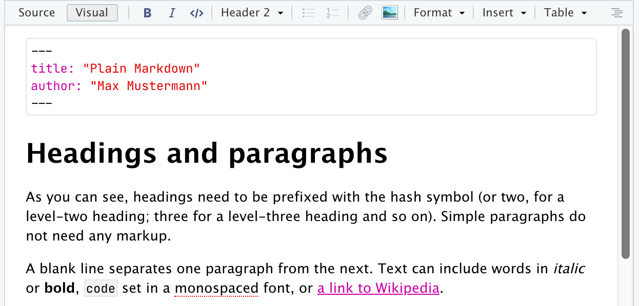
The first few lines (optional, located between the dashed lines) determine the front matter and options for the compiler, similar to the document preamble in LaTeX. For now, title, author and perhaps date are all we need. The syntax of these name-value pairs is called YAML so sometimes you will see this block being referred to as the “YAML header”.
---
title: Plain Markdown
author: Max Mustermann
---
# Headings and paragraphs
As you can see, headings need to be prefixed with the hash symbol (or two, for a level-two heading; three for a level-three heading and so on). Simple paragraphs do not need any markup.
A blank line separates one paragraph from the next. Text can include words in *italic* or **bold**, `code` set in a monospaced font, or [a link to Wikipedia](www.wikipedia.org).
# Lists
## Bulleted lists
There is no need to specify "environments" for bulleted or numbered lists; do make sure to separate them from the surrounding text with a blank line, however.
- Coffee
- Milk
- vegan
- non-vegan
- Tea
## Numbered lists
In numbered lists, you can mix different numbering patterns:
1. Coffee
2. Milk
a) vegan
b) non-vegan
3. Tea
# Special objects
You can include LaTeX-style formulas
$$ y_i = \beta_0 + \beta_1 x_i + \varepsilon_i $$
block quotes
> Almost all quotes from the internet are attributed to the wrong person. *Benjamin Franklin*
images (referenced by URL or file path)

or tables
| Variable | Description |
|------------------|------------------|
| `bill_length_mm` | Bill length (mm) |
| `bill_depth_mm` | Bill depth (mm) |8.2 Embedding code
To create a dynamic document, we need to include some code into our Markdown-formatted text. The file format that has traditionally been used to accomodate both in a single file is called R Markdown (.Rmd). Recently, Quarto (.qmd) has emerged as a versatile format to produce dynamic documents not only based on R but also Python and Julia. We will be using it here because it enables certain features for academic writing (such as cross-references and citations) by default. But don’t worry – the syntax is almost exactly the same as R Markdown.
8.2.1 Interactive exploration & rendering
After downloading and installing Quarto from quarto.org, re-start R Studio and create a new Quarto document with File > New File > Quarto Document.... Provide a title if you want, otherwise just accept the default values. What sets this document apart from the plain Markdown document we created earlier is the inclusion of executable code. Click inside the code chunk to verify that it is editable, add a + 1 and hit the green play button in the top right corner to see its output:
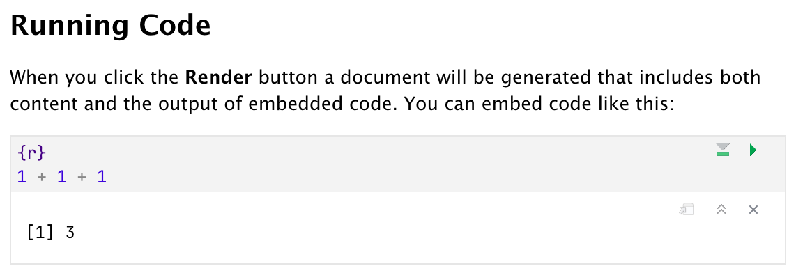
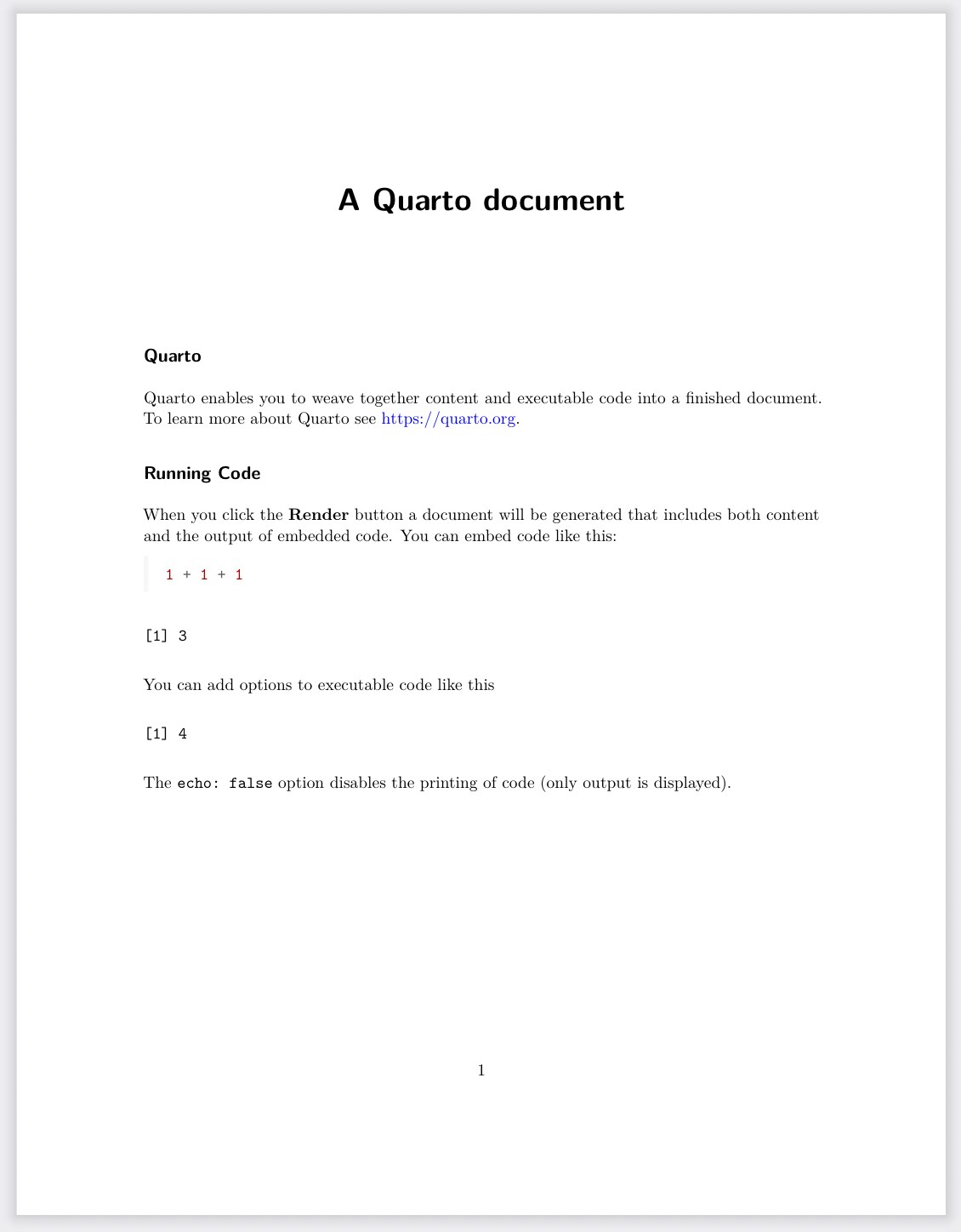
To create a new code chunk, click on Code > Insert Chunk. When you are satisfied with your interactive exploration, click on “Render” at the top of your editor. If you accepted the defaults earlier, your output will be HTML and shown in the Viewer pane. To produce a PDF document instead, change your YAML header to format: pdf and compile again. Your output should look like this:
8.2.2 Chunk options
We can tweak the behavior of each code chunk. If you look closely at the PDF output above, you will notice that the code output is shown for both chunks but the code itself is hidden for the second one. Chunk options are prefixed with a special comment marker, #|. Here, echo: false hides the code. Alternatively, we could use results: false to hide the output of the code chunk or eval: false to show code without executing it. A setup chunk that should quietly load packages goes well with include: false – it suppresses both the code, its output, messages and warnings. When a code chunk produces a plot, you can use the chunk options to hide or show the plot, adjust its dimensions or add a figure caption.
8.3 Academic writing
If you compare your lightweight Markdown document with your 3-page LaTeX preamble, you will rightly suspect that LaTeX has tricks up its sleeve that a dynamic document written in Markdown is not capable of. Part of this is by design: the simple Markdown format is intended to shift your focus on conducting and communicating your research, rather than fine-tuning the kerning between each pair of letters in the document.
But luckily, R Markdown/Quarto documents do come with features essential to writing an academic paper, such as cross-referencing and citations. Not only is the syntax much simpler than that of LaTeX; you will also never again have to compile four times in a row just to get the references right.
8.3.1 Footnotes
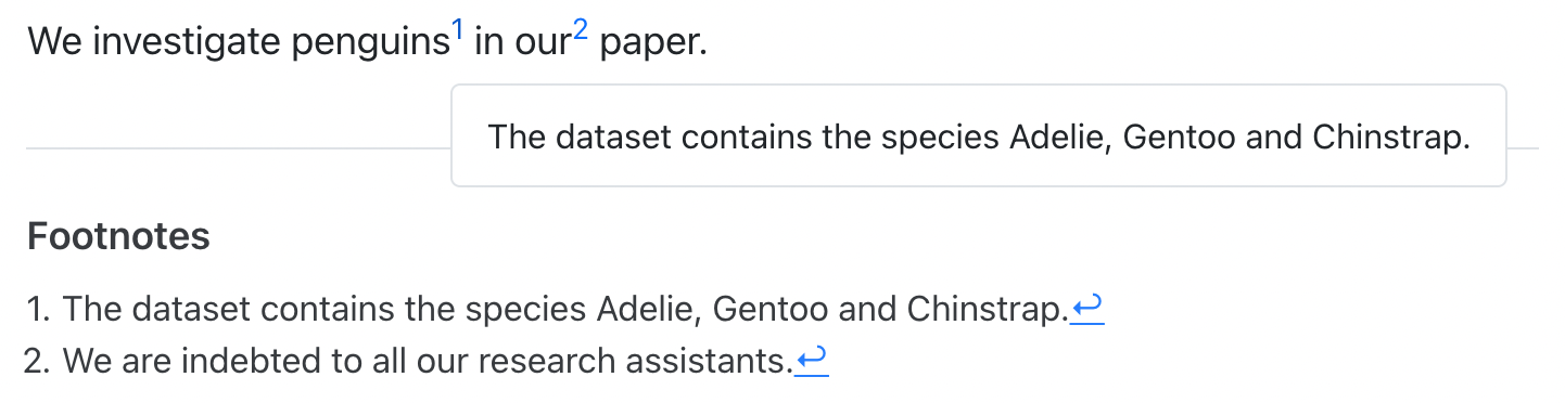
Footnotes are perhaps the epitome of academic writing. In Quarto, they come in two flavors: either as inline footnotes, similar to the way LaTeX handles them; or with a placeholder and a legend below. Note that the identifier a in the placeholder [^a] is arbitrary and could be a number or word instead.
We investigate penguins^[The dataset contains the species Adelie, Gentoo and Chinstrap.] in our[^a] paper.

[^a]: We are indebted to all our research assistants.
The output is the same for both notations. If you are exporting to HTML, footnotes will even pop up as you hover over them:
8.3.2 Cross-referencing
Each code chunk (output) can have a label to reference it. You can assign the label fig-speed (and a figure caption) to a scatter plot with
#| label: fig-speed
#| fig-cap: A non-ggplot
plot(cars)
To reference it in the text, add an @-sign in front of the label. This pair of commands is similar to \label{id} and \ref{id} in LaTeX but works for different output formats.
We can create plots without **ggplot2**, see @fig-speed.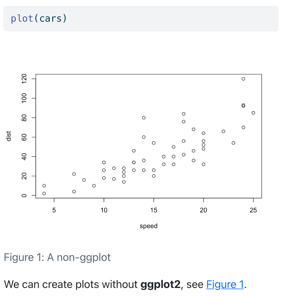
8.3.3 Citations
Let’s credit the authors of the palmerpenguins package that we have been using throughout this course. Similar to LaTeX, Quarto uses a .bib file to store citation entries. Save the following entry in a new file called lit.bib and add the line bibliography: lit.bib to your YAML header.
@Manual{penguins2020,
  title = {palmerpenguins: Palmer Archipelago (Antarctica) penguin data},
  author = {Allison Marie Horst and Alison Presmanes Hill and Kristen B Gorman},
  year = {2020},
  note = {R package version 0.1.0},
  url = {https://allisonhorst.github.io/palmerpenguins/},
}
You are now set to cite entries from this file. To reference our entry in the text, prefix the cite key (penguins2020) with the @-symbol, similar to cross-referencing. Add brackets if you want both the author and the year to appear in parentheses:
The package `palmerpenguins` was written by @penguins2020. The data is an example of Simpson's paradox [@penguins2020].
8.4 Caveats
The Quarto format (and dynamic documents in general) are a boon to reproducibility because prose and code never go out of sync. The syntax is simple and lends itself well to exporting to various formats. The default templates look great and conceal the nitty-gritty of the compilation process from the user.
But! The reduction in complexity is a double-edged sword. On the one hand, it allows us to focus on the actual research and ensure compatibility to various output formats; on the other hand, there might be specific features that are simply not implemented (yet).
For example, there are things in LaTeX that can only be achieved with a workaround, such as figure notes in addition to a figure caption. With Quarto, this becomes even harder to implement because it adds another layer between us and the final output.
Some strategies may help us in these cases. First, note that we can add raw LaTeX code in a Quarto document. When exporting to PDF, this works as expected; all other output formats will ignore this code. Second, you can use custom LaTeX templates or include LaTeX packages in the YAML header. You can even write a custom lua filter to customize your output further. As a last resort, you can always export the Quarto document as LaTeX and make manual adjustments before baking everything into a PDF.
8.5 Exercise
Complete the report on our exploration of the penguin data. Use this template as a starting point and try to replicate this finished document as closely as possible. You will have to add some formatting, broken cross-references and the bibliography. See the references below when you get stuck and try exporting to both PDF and HTML when you are done.
Answer
---
title: "Penguins"
author: Your Name Here
date: May 2022
format: pdf
bibliography: lit.bib
---

```{r}
#| label: load-packages
#| include: false

library(tidyverse)
library(palmerpenguins)
library(modelsummary)
library(fixest)
```

## Introduction

This report analyzes the `penguins` data from the **palmerpenguins** package. It will settle the longstanding debate in the literature whether there is a positive correlation between the variables

- bill length
- bill depth

According to @penguins2020, the dataset contains size measurements for `r nrow(penguins)` penguins from three species observed on three islands in the Palmer Archipelago, Antarctica.

## Distribution of species

We can determine the number of penguins for each species easily with functions from the **tidyverse** [@tidyverse2019]:

```{r}
#| eval: false
penguins %>%
  count(species)
```

However, using `datasummary_skim()` from the package **modelsummary** [@modelsummary2022] for the same task results in a nicely formatted table that is automatically embedded in this report.

```{r}
#| echo: false
penguins %>%
  select(species) %>%
  datasummary_skim(type = "categorical")
```

## Visual exploration

At first glance, there seems to be a *negative* correlation between bill length and bill depth, if anything. However, broken down by species the plot does support the notion of a positive correlation. This phenomenon (an effect that vanishes or reverses when groups are combined) is an example of [Simpson's paradox](https://en.wikipedia.org/wiki/Simpson%27s_paradox).

```{r}
#| label: fig-paradox
#| echo: false
#| warning: false
#| fig-cap: Simpson's paradox

ggplot(penguins, aes(bill_length_mm, bill_depth_mm)) +
  geom_point(aes(color = species, shape = species)) +
  scale_color_manual(values = c("darkorange","purple","cyan4")) +
  labs(
    title = "Bill length and bill depth",
    subtitle = "Dimensions for penguins at Palmer Station LTER",
    x = "Bill length (mm)", y = "Bill depth (mm)",
    color = "Penguin species",
    shape = "Penguin species"
  ) +
  theme_minimal()
```

In the next chapter, we will analyze the correlation depicted in @fig-paradox^[Labels should start with `fig-` for figures and `tbl-` for tables.] using linear regression.

## Statistical analysis

We formalize our model with the following equation:

$$ depth_i = \beta_0 + \beta_1 length_i + \varepsilon_i.$$
Results are displayed in @tbl-linreg.

```{r}
#| echo: false
#| warning: false
#| label: tbl-linreg
#| tbl-cap: Linear regression
mod <- feols(bill_depth_mm ~ bill_length_mm,
      data = penguins,
      split = ~species)

modelsummary(mod,
             vcov = "robust",
             stars = c("***" = 0.01, "**" = 0.05, "*" = 0.1),
             coef_omit = "Int",
             coef_rename = c("bill_length_mm" = "Bill length (mm)"),
             gof_map = c("nobs", "adj.r.squared", "vcov.type"))
```

## References
8.6 References and further reading
- Quarto documentation: Markdown Basics
- Quarto documentation: Cross References
- Quarto documentation: Citations & Footnotes